Simulation Based Assessment of Limited Sampling Strategies Reliability in the Estimation of the Area Under the Concentration-Time Curve

Simulation Based Assessment

of Limited Sampling Strategies

Reliability in the Estimation

of the Area Under the

Concentration-Time Curve

Leila K. Asl,

Fahima Nekka

Jun li

1 University of Montreal, Canada

2 Mathematics Research Centre, University

of Montreal, Canada

Corresponding author:Li J



C.P. 6128, Succ. Centre-ville, Montreal (Quebec), Canada, Math Research Center Ematiques, University of Montreal, Canada

Tel: +1 514 343 2026

Abstract

The area under the plasma drug concentration-time curve (AUC), representing the total drug exposure over time, is a common pharmacokinetic (PK) surrogate to inform the issue of therapy. Reliability of its estimation highly depends on the frequency of blood sampling. To reduce the cost and inconvenience of blood withdrawal, limited sampling strategies (LSS) have been proposed, with two main approaches for their development and implementation, whether the multiple linear regression-based LSS (R-LSS) or the Bayesian-based LSS (B-LSS). Regardless of the method used, evaluation of the predictive capacity of LSS is critical. Transferring an LSS between different clinical settings is an overlooked aspect, threatening thus the extension of its informed use. In the current paper, we study the reliability of a chosen LSS by proposing a hybrid approach that takes advantage of both R-LSS and B-LSS to analyze its robustness and success rate. The impact of variability on the LSS reliability is also investigated. As a result, we were able to show that our method enhances the selection of the best LSS and informs the associated risk to their transferability. This simulation-based methodology should be added to routine procedures of LSS development to complement traditional validations.

Keywords: Limited sampling strategies; Area under the curve; Multiple linear regression; Bayesian; Robustness; Transferability

Introduction

Therapeutic drug monitoring (TDM) is a routine clinical practice for drugs exhibiting significant inter- and intra- individual variability and narrow therapeutic ranges [1]. To optimize treatment efficacy and minimize toxicity, appropriate blood samples are collected for the estimation of therapeutic surrogates. The area under the plasma drug concentration-time curve (AUC) is a typical example [1-4]. Many methods have been proposed to estimate AUC. However, to be reliable, a rich number of samples

on individuals is usually needed for the use of these methods

[5]. In order to alleviate the associated burden of frequent blood withdrawal, limited sampling strategies (LSS), generally using 3 or less blood samples while keeping reasonable estimation accuracy were proposed and applied in clinical practice [6-9]. Two usual LSS approaches, the multiple linear regression (R-LSS) and the population pharmacokinetic (Pop-PK) model based empirical

Bayesian (B-LSS), are equally used for the estimation of AUC [10-12]. In the development of these LSS approaches, a reference dataset of dense sampling, with 6 to 10 blood samples of each individual, is usually provided [13]. Using the trapezoidal method, individual AUC is estimated and set as the reference AUC (AUC_ref). For R-LSS, different subsets of blood samples are tested using multilinear regression method with AUC_ref, and those with the closest predicted values to AUC_ref are identified. Noted as AUC , this prediction is expressed as



AUC

=

a a c a c

+

+

+

...

a c

where C_i are concentrations sampled at the chosen times t_i, and

a_i are the associated regression coefficients, i = 0, . . . k. For its

Pop-PK model is additionally required for the estimation of AUC. This model, considered as the prior acquired knowledge of drug characteristics, helps to improve the estimation, otherwise solely based on the observed drug concentrations. With the B-LSS method, the individual PK parameters are estimated using the empirical Bayesian approach, then used to predict

the individual’s drug concentrations and, consequently, the AUC [14]. One advantage of B-LSS over R-LSS is its flexibility in terms of sampling time deviations which are implicitly included in the framework of the Pop-PK modeling and the estimation of individual PK parameters. Nevertheless, the use of B-LSS can be hampered by the need for trained professionals and specialized software. This situation is however progressively changing since many PK software packages with user-friendly interfaces are now made available [8,11,12,15,16]. The predictive performance of LSS is generally evaluated through the calculation of their bias and precision [17]. Though these criteria inform a certain validity of the LSS, their predictive power and transferability should not be taken for granted when different patient subpopulations and contexts are involved [18]. This fact explains the variety of LSS reported for the same drug by different research groups [9,19]. When a specific LSS is intended to be used in a clinical setting or a population different from the one for which it has been originally established, the degree of its transferability or reproducibility should be of concern [9,20]. Traditionally, this was assessed clinically through a revalidation process using additional sub-population data [21]. However, running a separate clinical trial for each subpopulation can be unrealistic and even at a large risk of validation failure. To reduce this risk, a modeling-based approach using simulated data is a reasonable choice. We will refer to this transferability to indicate the reliability of a chosen LSS in different settings [9,16,22-24], which includes the robustness and the success rates as will be discussed in the current paper. By taking advantage of both R-LSS and B-LSS, we propose here a hybrid approach to measure the robustness of LSS with respect to the so-called between subject variability (BSV) and the residual variability (RV). Based on this, we will also propose several ways to assess the risk of an identified LSS. The current work concerns the methodology to evaluate the transferability of LSS, which is simulation based. The drug model is chosen from the literature and only used for an illustrative purpose. Therefore, the method we propose here can be easily applied to any drug scenarios with

similar needs.

Materials and Methods

Since our methodology is based on simulated data, a published Pop-PK model of cyclosporine (CsA) in clinical renal transplant patients [25] is chosen to illustrate our proposed evaluation procedure of LSS. First, using this model, a full sampling data set will be generated to serve the estimation of AUC_ref. Then,

different subsets of blood sampling with all possible combinations containing three time points are used to find the most performing LSS in terms of the closeness of their prediction of AUC to AUC_ref.

Once this selection is done, we will propose a simulation process for the assessment of their robustness. An analysis of the LSS robustness in the context of various variability will be investigated

as well. Moreover, the problem of how to assess the risk of an LSS in different settings, referred to here as the LSS success rates, will be discussed. These involved steps will be explained in more details below.

The Pop-PK model

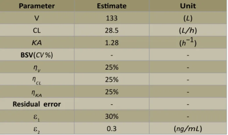
A one-compartment Pop-PK model with first-order elimination and absorption rate for cy-closporine (CsA) is chosen to illustrate our proposed approach [25]. Typical values of model parameters are used in this paper and summarized in Table 1.

In this model, BSV for PK parameters is described with the exponential model:

ij

ij je

η

θ =θ (2)

Where θ_ij is the jth _{PK parameter for the ith individual, θj is the}

typical value of the parameter, ηij is a random variable assumed to be normally distributed with zero mean and variance ω2. The unexplained variability RV is described using the additive and proportional model

(

)

1

obs pred

C = C × + ε + ε ₍₃₎

Where, C_obs and C_pred are the observed and predicted values of blood concentrations, respectively;

ε₁ and ε₂ are normally distributed random variables with zero mean and variances σ₁2 _{and σ}

22, respectively. For the sake of

simplicity, we take in this paper BSV as the average of η of the PK parameters and RV as the value of ε₁, since the impact of ε₂ on the

estimation of AUC is very small.

Simulated dataset of full sampling concentrations and the estimation of AUC_ref

Using the above Pop-PK model, 100 full sampling concentration datasets, with 60 subjects in each, were simulated. Using a previously reported protocol [11], 12 sampling points are chosen: 0, 0.5, 1, 1.5, 2, 3, 4, 8, 12, 15, 22 and 24 hours post dose. Using the trapezoidal method, AUC_ref was estimated for each of these

full sampling dataset. Identification of LSS

A number of 220 possible LSS, which are the combination results

Parameter Estimate Unit

V 133 (L)

CL 28.5 (L/h)

KA 1.28 (h−1)

BSV(C V %) -

-η_V 25%

-η_{C L 25%}

-η_KA 25%

-Residual error -

-ε₁ 30%

-ε₂ 0.3 (ng/mL)

V: apparent volume of distribution; C L: clearance; KA: first order

from three concentration-time points, were evaluated for their performance. For each dataset k, we performed a multiple linear regression in terms of the chosen combination of (C₁, C₂, C₃) and AUC_ref to determine the corresponding coefficients (a₁, a₂, a₃), which leads to the prediction of AUC_ref, _AUC :

 _{0 1 1 2 2 3 3}

AUC =a a C a C a C+ + + (4) The performance of the 220 LSS was evaluated using the 95th

percentile of the absolute values of relative prediction errors (95th

PAE%) [11,12]. For the given dataset k and the combination m, the relative error E_i, i = 1 • • • , 60, are calculated as

(5)

Where AUC_ref,i and AUCiare AUC_ref and AUC for ith individual, respectively. Then, 95th _{PAE% is estimated using the following}

formula

95th _{PAE% = 95}th _{percentile of the increasingly ordered set of {| E |}}

i. (6)

For each dataset k, the best N LSS among the 220 combinations in terms of 95th _{PAE% values are kept as appropriate candidates}

for AUC estimation. In the current paper, we considered the cases of N = 1 or N = 5.

Accordingly, for 100 simulated datasets, we thus have a list of 100 or 500 LSS that can be considered as the most promising LSS for the estimation of AUC. This list will be used to assess an LSS.

Reliability assessment of LSS

Using the above list, we can investigate the robustness of an LSS, and assess the risk of its use as well. We propose the following metrics for their estimations.

• Robustness: For an identified LSS in the list, its robustness refers to its frequency within the list. This can be explained by the fact that when an LSS appears the most in the identification process, it is the one which is likely to perform always the best, thus can be considered as the most robust.

• Absolute success rate: Given a 95th _{PAE% threshold Θ, for}

example 15% in the current paper, we can measure the rate that an identified LSS has 95th _{PAE% smaller than Θ within the 100}

simulated datasets. Mathematically, the absolute success rate of an LSS is given by

Absolute success rate = #{95th _{PAE%(LSS) < Θ}/100 (7)}

Where # is the number of occurrences. This rate can be interpreted as the confidence that one can have in an identified LSS to reach the expected accuracy when applied in a new setting.

• Relative success rate: We can also measure the rate that an identified LSS has the best performance compared to other LSS within the 100 datasets. For an identified best LSS_I, its relative success rate compared to another LSS_J can be defined as

Relative success rate = #{k : 95th _PAE%(LSS

J ) - 95th PAE% (LSSI ) > 0}/100 8)

Where # is the number of occurrences.

Analysis of LSS robustness for various variability

A different variability in PK parameters may change the predictive performance of an LSS. Hence we also estimate here the impact of the BSV and RV on the robustness of LSS. This allows a different angle of view to understand the risk of uncertainty of an LSS. Three levels (small, medium, high) of BSV and RV are tested. For BSV, the small, medium and high variability are 0-20%, 20-50% and 50-80%, respectively. For RV, three levels of 0-10%, 15-20% and 30-60% are used for the proportional component, and three levels of 0-0.1, 0.1-0.2 and 0.2-0.6 (ng/mL) for the additive component.

Software

The commercial software package MATLAB _{(2008b, The Math}

Works Inc, Natick, Massachusetts, USA) and NONMEM _(version

VII, Icon Development Solutions, Ellicott City, MD) were used for calculations and simulations.

Results

Robustness of the LSS

In the left panel of Figure 1, we display, in a 2-D contour plot heat map style, the LSS robustness in terms of different BSV and RV values. Figure 1A shows the robustness of the best (most frequent)LSS for N = 1. It can be observed that the robustness is very low even when BSV and RV values are very small, which makes the decision difficult regarding the appropriateness of these best LSS.

However, when N = 5, we have a larger list of LSS (500), from which a best LSS can be identified for each value of BSV and RV. It can be observed that there is a significant increase in robustness, as seen in figure 1B, making this situation more appealing. This increase is not homogeneous in terms of BSV and RV. For example, for medium variability as with BSV = 30% and RV = 20%, where the identified LSS is 172 (t₁ = 2h, t₂ = 4h, t₃ = 12h), its robustness is less than 50%. Nonetheless, when BSV is small (< 20%), we always have a high robustness (> 60%), regardless of RV. The estimation error of those LSS should be clinically acceptable. Figure 1C and D, represents the maximum estimation error for the best LSS, for N = 1 and N = 5, respectively. Contrarily to the robustness, there is no significant difference in the estimation error for the best LSS when small variability is present, as indicated in the lower left

square of Figure 1C and D.

Absolute success rate

In Figure 2, the left panel shows the robustness of LSS in a decreasing order, for three levels of BSV and RV, the middle panel displays the 95th _{PAE% of the most robust LSS of each level,}

compared to a threshold Θ = 15%, for 100 simulations or clinical settings. For BSV = 5% and RV = 10%, the most robust LSS noted 186 (t₁ = 3h, t₂ = 4h, t₃ = 8h) has a robustness larger than80 % and a full absolute success rate of 100%. Hence for a threshold of 15%, the LSS186 can besafely transferred to another setting. However, for BSV = 35% and RV = 20%, the most robustLSS, LSS₁₇₂ (t₁ = 2h, t = 4h, t = 12h), has a robustness of 49% and an absolute success

Figure 1 Robustness and maximum 95thP AE%. PAE-percentile absolute error; RV-residual variability; BSV-between subject variability.

Figure 2 Robustness, 95thP AE% and relative success rate of the best LSS. PAE, percentile absolute error; RV, residual variability; BSV,

rate of 23%, making it more susceptible to errors when applied in

different clinical conditions. Finally, for an extreme case of BSV = 40% and RV = 60%, LSS₁₈₆ is again the most robust, with more than 60%

of robustness but has null absolute success rate of 0%. If threshold of Θ = 20% is clinically acceptable, our conclusion for the LSS₁₇₂ can be changed, with a success rate of 95%, which may be acceptable. However, the conclusion for the third case remains unchanged.

Relative success rate

The right panel of Figure 2 shows the relative success rate of each of the most robust LSS of the left panel. In all cases, this success rate is higher than 50%. For BSV = 5% and RV = 10%, the most robust LSS noted 186 (t₁ = 3h, t₂ = 4h, t₃ = 8h) has a relative success rate of 60% and up, which supports its superiority as previously indicated. For the case of BSV = 40% and RV = 60%, LSS₁₈₆ still

Figure 3 Robustness vs. BSV for different RV. RV, residual variability; BSV, between subject variability.

distinguishes itself among the other LSS, though its absolute success rate makes it useless (the less worst). In the middle case of BSV = 35% and RV = 20%, we can see that LSS₁₇₂, has 53% of

relative success rate compared to its nearest competitor LSS₁₇₃ (t₁

= 2 h, t₂ = 4 h, t₃ = 15 h), making them almost equal in this aspect. However, the absolute success rate of LSS₁₇₃ is 20%, which is not far away from the one of LSS₁₇₂ which is 23%. In this case LSS₁₇₃ can be considered as an alternative for LSS₁₇₂.

Impact of different variability on the robustness

of LSS

Figure 3 and 4 display the robustness of best LSS in terms of BSV and BSV/RV, for increasing levels of RV. The results of Figure 3 show that, for any BSV, the robustness decreases with the increase in RV. However, for a fixed RV, the robustness decrease first when BSV increases, but then the trend is reversed at some point. We think this could be attributed to the different intrinsic natures of BSV and RV, while the former can be explained by the PK heterogeneity of the population and can be predicted by the Pop-PK model, while the latter refers to the unexplained part of the variability as a white noise of the model. Figure 4 informs

further by linking the ratio of BSV and RV to the robustness in presence of variability. We can see that, for all RV tested, the variation of robustness are almost in the same range and the mentioned trend changes around the point where BSV is almost double of RV.

Discussion

Limited sampling strategies have been proposed to reduce the invasiveness of therapeutic drug monitoring for drugs having large variability and narrow therapeutic ranges. A large number of studies have been performed for the selection of best LSS using data collected in a particular clinical setting. Many LSS have been identified to encompass a variety of compounds and populations. At the same time, new methodologies have been proposed; mainly using the multilinear regression or Pop-PK based empirical Bayesian approaches. Beyond the LSS selection, additional

aspects have recently been addressed, such as the impact of sampling time deviation on the prediction performance of LSS [12]. The LSS validation is an important issue. Many methods have been proposed regarding this respect, such as the Leave One out Cross Validation (LOOCV), Jackknife, bootstrapping, etc. All these methodologies are based on the use of a unique dataset, which is generally split into two parts: one for learning and the other for confirming. However, the limitation of these methods is that they are based on data collected bearing similar conditions. The generalizability and transferability of these developed LSS to another setting remains an open problem [9,16,18]. This is what we addressed in the current paper. In fact, there exist two main concerns: 1) how to facilitate the selection of the best LSS; 2) how to inform the associated risk for their extended use. To address these two points, we proposed here a hybrid approach that takes advantage of both R-LSS and B-LSS and can be used to evaluate the reliability of an LSS. Through a simulation approach and exemplified by a drug model, we here introduced the concept of LSS robustness and success rate. This enabled us to quickly identify a best LSS and quantitatively document its associated risk when the intent is to use it elsewhere. Since the variability is the major factor influencing the prediction capacity of LSS, we also studied the impact of different levels of BSV and RV on this prediction and found that the ratio of BSV and RV is a determinant factor. For illustration, we have chosen a relatively simple Pop-PK model with some modifications of the reported variability in order to easy our calculations. Doing so, we were able to quickly identify the problems and find the solutions. However, the proposed method can be easily adapted to more realistic situations and the developed procedure can be implemented within home developed software for its routine use in LSS development.

Acknowledgements

References

1 Touw DJ,Neef C, Thomson AH, Vinks AA (2005) Cost-Effectiveness of TherapeuticDrug Monitoring Com- mittee of the International Association for TherapeuticDrug M, Clinical T: Cost-effectiveness of therapeutic drug monitoring: A systematic review. Ther Drug Monit 27: 10-17.

2 Kahan BD (2002) Therapeutic drug monitoring of immunosuppressant drugs in clinical practice. Clinical Therapeutics 24: 1223-1223.

3 Wacke R, Rohde B, Engel G, Kundt G, Hehl EM, et al. (2000)

Comparison of several approaches of therapeutic drug monitoring of cyclosporinA based on individual pharmacokinetics. European Journal of Clinical Pharmacology 56: 43-48.

4 Wavamunno MD, Chapman JR (2008) Individualization of immunosuppression: Concepts and rationale. Current Opinion in

Organ Transplantation13: 604-608.

5 Yeh KC, Kwan KC (1978) A comparison of numerical integrating

algorithms by trapezoidal, La- grange, and spline approximation. J

PharmacokinetBiopharm6: 79-98.

6 Moore MJ, Bunting P, Yuan S, Thiessen JJ (1993)Development and validation of a limited sampling strategy for 5-fluorouracil given by

bolus intravenous administration. Ther Drug Monit 15: 394-399.

7 van Warmerdam LJ, ten Bokkel Huinink WW, Maes RA, BeijnenJH (1994)Limited-sampling models for anticancer agents. J Cancer Res Clin Oncol 120: 427-433.

8 Panetta JC, IaconoLC,AdamsonPC,Stewart CF (2003) The importance

of pharmacokinetic limited sampling models for childhood cancer

drug development. Clin Cancer Res 9: 5068-5077.

9 Ting LS, Villeneuve E, Ensom MH (2006) Beyond cyclosporine: A systematic review of limited sampling strategies for other immunosuppressant. Ther Drug Monit 28: 419-430.

10 SpragueDA, EnsomMH (2009) Limited-sampling strategies for ant i-infective agents: Systematic review. Can J HospPharm62: 392-401.

11 Sarem S, Li J, Barri`ere O, Litalien C, Th'eoret, et al. (2014)Bayesian approach for the estimation of cyclosporine area under the curve using limited sampling strategies in pediatric hematopoietic stem cell transplantation. Theor Biol Med Model 11: 39.

12 Sarem S, Nekka F, Ahmed, S I, Litalien C, Li J (2015) Impact of sampling

time deviations on the prediction of the area under the curve using regression limited sampling strategies. Biopharm DrugDispos. 13 DasguptaA (2012) Therapeutic drug monitoring: Newer drugs and

biomarkers (1st _{edn). Elsevier, USA.}

14 Abd Rahman A, Tett S, Staatz C (2014) How Accurate and

PreciseAre Limited Sampling Strategies in Estimating Exposure to Mycophenolic Acid in People with Autoimmune Disease?

Clinical Pharmacokinetics53: 227-245.

15 Loh GW, Ting LS, Ensom MH (2007) A systematic review of limited sampling strategies for platinum agents used in cancer chemotherapy. Clin Pharmacokinet46: 471-494.

16 van der Meer AF,MarcusMAE, TouwDJ,Proost JH,NeefC (2011) Optimal Sampling Strategy Development Methodology Using

Maximum A Posteriori Bayesian Estimation. TherapeuticDrug Monitoring 33: 133-146.

17 Sheiner LB, Beal SL (1981) Some Suggestions for Measuring

Predictive Performance. Journal of Pharmacokinetics and

Biopharmaceutics 9: 503-512.

18 Barraclough KA, Isbel NM, Franklin ME, Lee KJ, Taylor PJ, et al. (2010) Evaluation of limited sampling strategies for mycophenolic acid after mycophenolate mofetil intake in adult

kidney transplant recipients. Ther DrugMonit 32: 723-733.

19 David OJ, Johnston A (2001) Limited sampling strategies for

estimating cyclosporin area under the concentration-time curve: review of current algorithms. Ther DrugMonit 23: 100-114.

20 Op den Buijsch RA, van de PlasA,StolkLM, Christiaans MH, van

Hooff JP, et al. (2007) Evaluation of limited sampling strategies

for tacrolimus. Eur J Clin Pharmacol 63: 1039-1044.

21 Suarez-Kurtz G, Ribeiro FM, Vicente FL, Struchiner CJ (2001) Development and validation of limited- sampling strategies for

predicting amoxicillin pharmacokinetic and pharmacodynamic

parameters. Antimicrob Agents Chemother 45: 3029-3036.

2 2 ( 1994) Drugs Directorate Guidelines, Acceptable Methods.

Health ProtectionBranch-Health and Welfare Canada: 20-22.

2 3 ( 1994)Text on Validation of Analytical Procedures. ICH

Harmonized Tripartite Guideline prepared within the Third

International Conference on Harmonization of Technical

Requirements for the Registration of Pharmaceuticals for Human

Use (ICH).

2 4 ( 1996) Validation of Analytical Procedures: Methodology.

ICH harmonized Tripartite Guideline pre- pared within the Third

International Conference on Harmonization of Technical Requirements for the Registration of Pharmaceuticals for Human Use (ICH) : 1-8.

25 Wu KH, Cui YM, Guo JF, Zhou Y, Zhai SD, et al. (2005) Population pharmacokinetics of cyclosporine in clinical renal transplant