CSC473: Advanced Algorithm Design Winter 2018
Week 7–8: Linear Programming
Aleksandar Nikolov
1
Introduction
You have seen the basics of linear programming in CSC373, so much of this should be review material.
A linear program (LP for short) is an optimization problem in which the constraints are linear inequalities and equalities, and the objective function is also linear. There are many equivalent standard forms for LPs. We will use the following form for a maximization problem:
maxc|x s.t. Ax≤b x≥0
Let us explain the notation a bit. HereA is an m×nmatrix (i.e. m constraints and nvariables) and bis an m×1 column vector;cis an n×1 column vector which encodes the objective function and c|is its transpose; xis an n×1 column vector which contains the variables we are optimizing
over. The inequalities between vectors mean that the inequality should hold in all coordinates simultaneously. The value of this LP is the minimum value of the objective c|x achieved subject to x satisfying the constraints. Any value of x that satisfies the constraints x ≥0 andAx ≤b is called feasible. The set of feasible x is called the feasible set or feasible region of the LP. When the feasible set is empty, the LP is calledinfeasible. The maximum value of the objective c|xover feasible xis the optimal value of the LP. If this maximum is infinity, i.e. for anyt∈R there exists a feasiblex s.t. c|x≥t, then the LP is calledunbounded.
Analogously, the standard form we use for a minimization problem is: minc|x
s.t. Ax≥b x≥0
Just for concreteness, let us write a tiny example of a linear program:
minx1+x2+x3 (1) s.t. x1+x2≥1 (2) x2+x3≥1 (3) x1+x3≥1 (4) x1, x2, x3≥0 (5)
This LP corresponds to b=c= 1 1 1 , A= 1 1 0 0 1 1 1 0 1 .
Exercise 1. Let G= (V, E) be a directed connected graph, let c:E→R be the capacities, and let
s, t ∈V be, respectively, a source and a target vertex. Use linear programming to decide whether there exists a flow f :E →R from sto t of value 1 that strictlyrespects the capacity constraints, i.e. such that for all e∈E we have 0 ≤f(e)< c(e). Write a linear program which is feasible and has positive value if such a flow exists, and is infeasible or has value0 if no such flow exists.
2
Geometric View
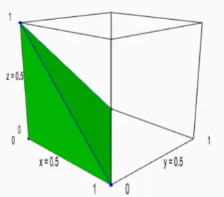
A geometric view is very useful in understanding LPs. Let us plot the the points (x1, x2, x3)
satisfying the following system of inequalities:
x1+x2+x3≤1 (6)
x1, x2, x3 ≥0 (7)
Figure 1 shows the points satisfying these inequalities. Let us introduce some terminology. Recall
Figure 1: A polytope in 3 dimensions.
the equation of a line in two dimensions a1x1+a2x2 =b, which can be written in vector notation
asa|x=b. Similarly, in three dimensions, the equation of a plane isa
1x2+a2x2+a3x3=b which
in vector notation isa|x=b. In general the set{x∈Rn:a|x=b}, where Rn is the set of vectors
with nreal coordinates, is called a hyperplane. For some geometric intuition, let us mention that any line lying in the hyperplaneH ={x∈Rn:a|x=b}which intersects the line `={ta:t∈
R}
is perpendicular to`.
Exercise 2. If ` is the line `=`={ta:t∈R} and H is the halfspace H ={x ∈Rn :a|x=b},
determine the pointz=`∩H. Show that any line`0 ={z+tv:t∈R}contained inH must satisfy
The set {x ∈ Rn : a|x ≤ b} is called a halfspace, and {x :∈
Rn : a|x = b} is its supporting
or bounding hyperplane. To get a picture of a halfspace, notice that in 2 dimensions a halfspace is everything on one side of a line, and in 3 dimensions it’s everything on one side of a plane. See Figure 2 for examples. The figure satisfying equations (6)–(7) is the intersection of the four
Figure 2: Halfspaces in 2 and 3 dimensions. halfspaces{x∈R3 :x
1+x2+x3≤1},{x∈R3 :x1 ≥0},{x∈R3 :x2 ≥0},{x∈R3:x3≥0}. A
set which is the intersection of halfspaces is called apolyhedron. We can always write a polyhedron P asP ={x∈Rn:Ax≤b}for some matrix Aand vectorb.
A polyhedron P ⊆Rn is unbounded when there exists a point x∈P and a direction v ∈
Rn such
that for every t≥0, x+tv ∈ P. (A set of the type {x+tv :t≥ 0} is called a ray.) Intuitively, this means that there is a starting point and a direction in which we can go infinitely long. For example, the polyhedron satisfying the inequalities
−x1+ 2x2≥1
2x1−x2≥1
is unbounded, because the ray {(1,1) +t(1,1) : t≥ 0} is contained in it (see Figure 2). When a polyhedron is bounded (i.e. not unbounded), it is called apolytope. For example, the set in Figure 1 is a polytope.
Figure 3: Unbounded polyhedron
Notice the structure of the polytope in Figure 1: its surface “consists” of 4 triangles glued to each other (we see three of them and one is hidden from view). These triangles are called the facets of the polytope. The triangles two by two along a line segment: these line segments (6 of them) are
called the edges of the polytope. Finally, the triangles meet three by three at a point: these points (4 of them) are called the vertices of the polytope.
Formally, a face of a polyhedron P = {x : Ax ≤ b} ⊂ Rn is a set of the type F = {x : Ax ≤ b} ∩ {x :aix =bi ∀i∈ S}, where ai is the i-th row of the matrixA, and S is some subset of the rows ofA. Usually, we also assume that F 6=∅. Let us use the notationSF for the set of allisuch that aix = bi for all x ∈ F. When the dimension of the span of {ai : i ∈ SF}, or, equivalently, the rank of the submatrix AF of A consisting of the rows of A indexed by SF, is n−j, we say that F is a face of dimension j, or, in short, a j-face. The dimension of the polytope P itself is defined similarly: SP is the set of all i such that aix =bi for all x ∈ P, and the dimension of P is n−rank AP, where AP is the submatrix of A consisting of the rows indexed by SP. We sayP is full-dimensional when its dimension is n, i.e., when SP = ∅. The faces of dimension one lower than the dimension of P are called facets; the 1-faces are called edges, and the 0-faces are called vertices. To see the reason behind this definition of the dimension, let us take some point x which is strictly insideF, i.e., not in any face strictly contained inF, and letW ={z:AFz= 0} be the nullspace of AF. Then for any i6∈ SF, aix < bi, and if we take any z ∈ W, and a small enough constant ε > 0, the point x0 =x+εz still satisfies aix0 = bi for all i∈ SF, and aix0 < bi for all i6∈SF. Since, by the rank-nullity theorem, W is a subspace of dimension n−j, this means that there is an (n−j)-dimensional ball around x which lies insideF, which is why we say that F is (n−j)-dimensionl.
Exercise 3. Let v be a vertex of the polytopeP ={Ax≤b} and letS be the setS ={i:aiv=bi}. Give a formula forv in terms of S, A, andb. Give an upper bound on the number of vertices of P in terms of the dimensions of the matrix A.
For example, let P be the polytope satisfying the constraints (6)–(7). The triangle with vertices (1,0,0), (0,1,0), and (0,0,1) is a facet (and also a 2-face), and can be written as F = P ∩ {x1+x2 +x3 = 1}. The edge e connecting (1,0,0) and (0,1,0) is a 1-face, can be written as
e = P ∩ {x1 +x2 +x3 = 1, x3 = 0}. The vertex v = (0,0,1) is a 0-face, can be written as
v=P ∩ {x1+x2+x3= 1, x1 = 0, x2 = 0}. See Figure 4 for a 2-dimensional example.
P H1 F v F1 F2
Figure 4: Faces of a 2-dimensional polytope (i.e. a polygon). The 1-faceF is the intersectionP∩H. The vertexv is the intersection of the two facetsF1 andF2.
A polytope is determined by its vertices in a strong sense. To make this precise, we define the notion of a convex hull: the convex hull of the pointsv1, . . . , vN ∈Rn is the set
For some geometric intuition, we mention that the convex hull of two pointsv1, v2is simply the line
segment connecting them; the convex hull of three points v1, v2, v3 is the triangle with the points
as its vertices. In general, conv{v1, . . . , vN} is the smallest polytope that contains v1, . . . , vN.
Exercise 4. Show that ifv1, . . . , vN belong to the polytopeP ={Ax≤b}, thenconv{v1, . . . , vN} ⊆ P.
We have the following basic theorem. You will not be responsible for the proof, but we include it for your interest.
Theorem 1. A polytope P with vertices v1, . . . , vN satisfies P = conv{v1, . . . , vN}.
Proof Sketch. Let P ={x :Ax≤b}, and let Sx ={i :aix = bi}. Let Ax be the submatrix of A consisting of the rows indexed by Sx. We will show that every x ∈P is in the convex hull of the verticesv1, . . . , vN; i.e. we will show that there exist non-negative λ1, . . . , λN, which sum to 1, and give λ1v1+. . .+λNvN =x. This will show that P ⊆conv{v1, . . . , vN}. The other containment conv{v1, . . . , vN} ⊆P follows from Exercise 4.
The proof is by induction onn−rank Ax. In the base case we have rank Ax =n, and thenx is a vertex of P, so there is nothing to show. Assume then that rank Ax < n. Then there exists some vectory∈Rnfor which A
xy= 0. Let
α= max{α0:x+α0y∈P}, β= max{β0 :x−β0y∈P}.
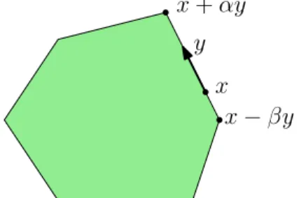
These maxima must exist, becauseP is bounded. Pictorially, we are finding some directiony such that we can walk a positive distance in the direction ofy and stay inside P, and also we can walk a positive distance in the direction of −y and also stay inside P. This is illustrated in Figure 5. The main point of the proof is that the furthest points we can travel in these directions lie in lower dimensional faces ofP.
x y x+αy
x−βy
Figure 5: Illustration of the inductive step in the proof of Theorem 1 It is easy to check that
α= min bi−aix aiy :aiy >0 , β = min bi−aix |aiy| :aiy <0 .
From these expressions it is clear that α, β > 0. Moreover, there exists some i+ (any one one
Sinceai+y >0,ai+ cannot be in the linear span of{ai:i∈Sx}. Therefore, rankAx+αy >rankAx.
Analogously, we can show rankAx−βy>rankAx. By induction, we have x+αy=λ01v1+. . .+λ0NvN,
x−βy=λ001v1+. . .+λ00NvN,
for non-negativeλ0, λ00 such thatλ01+. . .+λ0N =λ001+. . .+λ00N = 1. Then, we can write x= αβ
α(α+β)(x+αy) + αβ
β(α+β)(x−βy). We can then define λi = α(ααβ+β)λ0i+β(ααβ+β)λ00i for all i, and we are done.
Let us now interpret LPs geometrically. Let’s take a maximization problem max{c|x:Ax≤b, x≥
0}. The feasible set P ={Ax≤b, x≥0}is a polyhedron. We can view the objective cas a vector pointing from the origin 0 to the point with coordinates c. So the LP asks us to find the point in P which is the farthest out in the direction of the vector c. For example, consider the LP which maximizes the value of x3 subject to the constraints (6)–(7). This LP corresponds to finding the
point furthest along the direction of the vector pointing from the origin to (0,0,1) in the polytope in Figure 1. I.e. we want to find the point in the polytope which is highest up. Visually, it’s clear that the optimal solution of the LP is the point (0,0,1). Notice that the optimal solution is a vertex. This is a general phenomenon, and in fact follows easily from Theorem 1.
Corollary 2. If max{c|x:Ax≤b, x≥0} is an LP whose feasible region P ={x:Ax≤b, x≥0}
is a polytope, then the LP has an optimal solution which is a vertex of P.
Proof. Letxbe any optimal solution of the LP. By Theorem 1, we can writex=λ1v1+. . .+λNvN,
whereλ≥0,λ1+. . .+λN = 1, andv1, . . . , vN are the vertices ofP. We have
c|x=λ1c|v1+. . .+λNc|vN ≤λ1 N max i=1 c |v i+. . .+λN N max i=1 c |v i = N max i=1 c |v i.
Therefore any vertex vi achieving the maximum on the right hand side is also an optimal solution of the LP.
Note that if the LP has many optimal solutions, then not all of them will be vertices, but there always will be at least one which is a vertex. For example, suppose we maximize the objective x1+x2+x3 subject to the constraints (6)–(7). Then one optimal solution is (1/3,1/3,1/3), which
is not a vertex. Nevertheless, the vertices (1,0,0), (0,1,0), and (0,0,1) are all optimal solutions as well.
3
Simplex and Ellipsoid Algorithms
After this introduction to geometry, we will describe, on a very high level, two algorithms for solving linear programs. We will only describe these algorithms geometrically, and will not worry about the implementation details, which are far from trivial. Our goal is just to get the geometric intuition behind the algorithms, which are both quite beautiful.
3.1 Simplex Algorithm
The idea of the simplex algorithm is simple. Suppose we want to solve the LP max{c|x : Ax≤
b, x ≥0}. Let P = {x ∈ Rn : Ax≤ b, x ≥ 0} be the feasible region. As we already saw, P is a polyhedron; for simplicity, let’s assume that it is also a polytope. The simplex algorithm starts at some vertexx(0)ofP. (Getting a vertex to start from is not always easy. However, for many LPs in practice there is a clear choice.) LetN(x(0)) be the set of neighboring vertices to x(0), i.e. vertices y such that there is an edge of P connecting x(0) and y. The algorithm picks an element x(1) of N(x(0)) such that c|x(1) > c|x(0). Then this process continues: at each step t, the algorithm
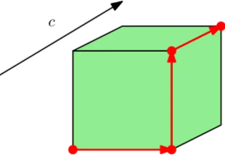
computes a new vertexx(t) from x(t−1) by picking a vertex x(t) ∈N(x(t−1)) s.t. c|x(t) > c|x(t−1). We stop once the objective function cannot be improved anymore: in this case, ifP is a polytope, i.e. bounded, we have found an optimal solution to the LP, and, moreover, the solution is a vertex. In Figure 6 we show a run of the simplex algorithm on a 3-dimensional cube.
c
Figure 6: The simplex algorithm, run on a cube. We have swept many things under the rug:
• How do we find a starting vertexx(0)?
• How do we know if P is bounded?
• How do we compute the neighboring vertices of x(t)?
• If there are multiple options forx(t)which improve the objective value, which one do we pick? An very interesting question is the running time of the simplex algorithm. While the algorithm seems to perform really well in practice, for essentially all known variants of it the worst-case complexity is exponential. Here by “variants” we mean the rule used to pick a neighborx(t)ofx(t−1), when there are multiple options. Such rules are known aspivot rules. It remains an important open problem to find a pivot rule for which the simplex algorithm runs in time polynomial in the number of variables and the number of constraints, or to show that no such pivot rule exists. One way to show that no such pivot rule exists would be to give a counterexample to the polynomial Hirsch conjecture: come up with a polytopeP ⊂Rn, determined by m constraints, and two vertices x, y
of P such that the shortest path between x andy has exponentially many edges. 3.2 The Ellipsoid Algorithm
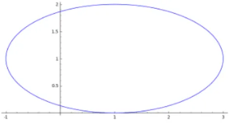
The ellipsoid algorithm is based on very different ideas. In order to understand the algorithm, we need to take another detour into geometry, and introduce ellipsoids. Recall that in two dimensions
we can write an ellipse (with major axes parallel to the coordinate axes) as {x ∈ R2 : a2(x 1−
y1)2 +b2(x2−y2)2 ≤1}. See Figure 7 for an example withy1 =y2 = 1, a= 1, b = 2. In higher
Figure 7: An ellipse in 2 dimensions
dimensions we define an ellipsoid as the set E(y, M) = {x ∈ Rn : (x−y)|M|M(x−y) ≤ 1}, where M is an n×n invertible matrix, andy ∈Rn is the center of the ellipsoid. When M = 1rI (I here is the identity matrix) we write B(y, r) = E(y, r−1I); such en ellipsoid is called a ball of radius r. In 2 dimensions, this is a disc of radius r, and in 3 dimensions it is a 3-dimensional ball of radius r. Indeed, in 2 dimensions, B(y, r) = {(x1, x2) :
p
(x1−y1)2+ (x2−y2)2 ≤ r}, and
in 3 dimensions B(y, r) = {(x1, x2, x3) : p
(x1−y1)2+ (x2−y2)2+ (x3−y3)2 ≤ r}. In general
E(y, M) = y +M−1B(0,1), where M−1B(0,1) = {M−1z : z ∈ B(0,1)}. In other words, an ellipsoid is the image of the unit ball under a translation and a linear map. (The combination of a translation and a linear map is known as anaffine map or an affine transformation.)
Here we are going to focus on the feasibility problem: given a polytope, described by inequalities, decide if it is empty. There are several ways to reduce solving LPs to this feasibility problem, and possibly the simplest one is based on binary search. Suppose we have the LP
maxc|x s.t. Ax≤b x≥0
and let P = {x ∈ Rn : Ax≤ b, x ≥ 0} be its feasible region. It’s usually easy to get two values v, V ∈R such that the optimal solution of the LP is guaranteed to be in the interval [v, V]. Let Qt=P∩ {x∈Rn:cTx≥t}. For any value oft,Qt is a polytope, and solving the LP is equivalent to finding the largest t such that Qt6=∅. If we have an efficient procedure to solve the feasibility problem, we can get arbitrarily close to this optimalt by doing binary search on [v, V].
Let us then focus on the feasibility problem: given a polytope Q = {x ∈ Rn : Dx ≤ e}, decide if it is empty or not. In fact, we need a little more information. We need a number R so that Q⊆B(0, R). We also need another numberr < R, and we need the “promise” that either Q=∅, or there exists a center y ∈ Rn for which B(y, r) ⊆ Q. R can be computed from the description of Q. In order to satisfy the promise, we compute another polytope ˜Q, based on Qsuch that if Q is empty, then ˜Q also is empty, and if Q is not empty, then ˜Q contains a ball of radius r. In the description of the algorithm below, we assume that we have substitutedQwith ˜Qand the promise is satisfied.
We can finally describe the algorithm, which is actually quite intuitive. At each time step t, the algorithm keeps an ellipsoid Et=E(yt, Mt) so that Q⊆Et. Initially,E0 =B(0, R). At stept, the
terminates. Otherwise, we can find some constraint ofQ violated by yt−1, i.e. some row di of the matrix D so that diyt−1 > ei. Let Hi− be the halfspace {x ∈ Rn : dix ≤ ei}. We know that Q⊆Et−1∩Hi−. Moreover,Et−1∩Hi− has volume1 at most half that ofEt−1, because it does not
contain the center ofEt−1. Then we can compute a new ellipsoidEtwhich containsEt−1∩Hi−, and, therefore, contains Q as well. While Et will have volume slightly larger than that of Et−1∩Hi−, we can still show that its volume is strictly less than that of Et−1. Therefore, the volume of the
ellipsoidsE0, E1, E2, . . . keeps decreasing, and after a while we know that the volume ofEt is less than that of any ball of radius r. This means that there is no y∈Rn such that B(y, r) ⊆Q, and, by the promise we had on r and Q, we know thatQ=∅.
A step of the algorithm is illustrated in Figure 8.
P E0 y0 H− i P E1 E0 y1
Figure 8: One step of the ellipsoid algorithm.
Unlike the simplex algorithm, the ellipsoid algorithm has worst-case running time polynomial in the number of bits needed to describe the LP. In fact, it was the first such algorithm, and of significant theoretical importance. However, in practice the simplex algorithm usually performs quite well, while the ellipsoid algorithm is not really practical. It seems that the simplex algorithm, unlike the ellipsoid algorithm, achieves its worst-case performance only on very special instances. Moreover, the ellipsoid algorithm needs to perform algebraic operations down to very high precision, which slows it down significantly.
There is another family of algorithms which we will not mention: interior point methods. These algorithms reduce solving an LP to solving an unconstrained, but non-linear optimization problem. Their name comes from the fact that, geometrically, they trace a path towards the optimal solution inside the feasible region, rather than on the boundary, as the simplex algorithm. The most efficient interior point methods give the best of both worlds: their worst-case running time is polynomial, and they also tend to perform well in practice. Interior point methods are currently a very active area of research.
Finally, there are algorithms designed to solve specific LPs. In fact you already have seen such algorithms: the maximum flow problem can be written as an LP, and the different variants of the Ford-Fulkerson algorithm solve this LP. Soon we will see other examples, when we talk about
1There is a natural way to generalize 2-dimensional area and 3-dimensional volume ton-dimensional volume. The idea is that that a set inRnof volume 1 has as much “space” inside of it as the side 1 cube{x∈Rn: 0≤xi≤1∀i∈
primal-dual algorithms. While these algorithms do not work for general LPs, they are usually simple and efficient.
4
Duality
Consider the LP in (1)–(5). If you wanted to convince someone that the optimal value of this LP isat most 3/2, then all you need to do is to present them with a feasible solutionx which achieves this value. For example, you can take x1 = x2 = x3 = 1/2. However, how would you convince
someone that this is in fact an optimal solution, i.e. that the optimal value of the LP is alsoat least 3/2? No single feasible solution proves that, because the optimal value of the LP is the minimum over all feasible solutions. A powerful idea is to show that the inequality x1+x2+x3 ≥ 3/2 is
implied by the constraints of the LP. In this case this is actually quite easy. You can add up the three constraints (2)–(4) and you get the new (implied) constraint 2x1+ 2x2+ 2x3≥3. Now divide
both sides of this inequality by 2 and you are done.
For another example, let us take the LP which maximizes x3 subject to the constraints (6)–(7).
As we mentioned before, geometrically, it seems clear that the optimal value is 1. To show more formally that the value is at least 1, we just need to exhibit a feasible solution: x1 = x2 = 0 and
x3 = 1. To show that x3 ≤ 1, observe that (6) and the non-negativity constraints (7) imply that
x3 ≤x1+x2+x3≤1.
Let us try to formalize this technique, and put it in as general terms as possible. Recall that we write a generic maximization LP as:
maxc|x (8)
s.t.
Ax≤b (9)
x≥0 (10)
Let us call this theprimal LP. To it corresponds a dual LP:
minb|y (11)
s.t.
A|y≥c (12)
y ≥0 (13)
Notice that in this program the variables arey ∈Rm, wheremis the number of rows of the matrix
A. To see how we this LP corresponds to what we did above, observe that A|y, for any y ≥ 0 is a non-negative combination of the left hand sides of the constraints Ax ≤ b, and b|y is the corresponding non-negative combination of the right hand sides.
Exercise 5. Write the dual linear program to the following linear program: maxc|x
s.t. Ax=b x≥0
The following theorem, known as the weak duality theorem, proves that the dual LP indeed gives upper bounds on the optimal value of the primal LP.
Theorem 3 (Weak Duality). Let x satisfy the primal constraints (9)–(10), and let y satisfy the dual constraints (12)–(13). Then c|x≤b|y.
Proof. The main observation we use is that if u, v, w ∈Rn, and u ≥ v, w ≥ 0, then u|w ≥v|w.
(Make sure you understand this.)
Using c ≤ A|y and x ≥ 0, we have c|x ≤ y|Ax. In turn, using Ax ≤ b and y ≥ 0, we have y|Ax≤y|b. Combining the two inequalities proves the theorem.
A surprising, important, and very powerful fact is that this simple way to bound the optimal value of an LP gives a tight bound for every LP:
Theorem 4(Strong Duality). Suppose that the primal program(8)–(10)and the dual program (11)– (13) are both feasible. Then their optimal values are equal.
The heart of the proof of this theorem is a useful lemma, known as Farkas’s lemma. There are many different version of it. We will state one which is amenable to a geometric proof.
Lemma 5 (Farkas’s Lemma). For anym×nmatrixA and any m×1vector b, exactly one of the following two statements is true:
1. There exists a x∈Rn,x≥0, such thatAx=b. 2. There exists a y∈Rm such that A|y≤0 and b|y >0.
You can view Farkas’s lemma as characterizing when the constraintsAx=b, x≥0 are (in)feasible: there either exists a simple “obstacle” to feasibility, i.e. a vectorysuch thatA|y≤0 andb|y >0, or the constraints are feasible. It should be clear that the existence of such ay contradicts feasibility of Ax =b, x ≥0. The lemma shows that this is the only possible reason the constraints are not feasible.
Exercise 6. Prove that if there exists a vector y∈Rm such thatA|y≤0 and b|y >0, then there
exists no x≥0 such that Ax=b.
It may be helpful to see an analogue to Farkas’s lemma for linear equalities.
Exercise 7. Using what you know from linear algebra, prove that for anym×n matrixAand any m×1 vector b, exactly one of the following two statements is true:
1. There exists a x∈Rn such that Ax=b.
2. There exists a y∈Rm such that A|y= 0 and y|b6= 0.
Proof of Lemma 5. From Exercise 6, only one of the two statements can be true. It only remains to show that if the first statement is not true, the second must be. I.e. we need to show that the only possible reason thatAx=bis not feasible is that there exists a yas in the second statement.
In the proof, we will adopt a geometric viewpoint. Let C ={Ax:x ≥0}. Such a set is called a cone. If the first statement of the Lemma does not hold, then we have thatb6∈C. Observe that if A|y ≤0, then every z ∈C satisfies y|z =y|Ax ≤0. Then, geometrically what we are trying to show is that if b6∈C, then there exists a hyperplane H ={z:y|z = 0} through the origin, such that all ofC is on one side ofH, and b is on the other. This is a simple geometric certificate that b6∈C, and a special case of thehyperplane separation theorem. See Figure 9 for an illustration.
b H y C a1 a2
Figure 9: An illustration of the Farkas lemma for a 2 by 2 matrix A= (a1, a2).
In the proof we will work with the (Euclidean) norm k · k defined for a vector z ∈ Rm by kzk =
√
z|z=p
z12+. . .+z2
m. Notice that in two or three dimensions this gives the usual distance from the origin 0 toz. It is clear from the definition thatkzk>0 for every nonzero z, and k0k= 0. Let nowzbe the closest point inC tob: z= arg min{kb−z0k2 :z0 ∈C}. We will need the following important claim.
Claim 6. We have z|(b−z) = 0.
Proof. If z = 0 the claim is trivially true, so let us assume z 6= 0. Let us write the function f(t) =kb−tzk2. From the definition of z, we have that f(1) is a minimum of this function over
t≥0, and, thereforef0(1) = 0 by elementary calculus. Expanding f(t), we have f(t) = (b−tz)|(b−tz) =kbk2+t2kzk2−2tz|b.
Therefore,f0(t) = 2tkzk2−2z|b, and f0(1) = 0 implies 2z|(z−b) = 2kzk2−2z|b= 0. Multiplying
both sides by −1/2 givesz|(b−z) = 0.
Geometrically, the claim means that zand b−z must form a right angle.
Becauseb6∈C, we must havekb−zk2 >0: otherwiseb−z= 0, sob=z∈C, a contradiction. Let
us definey=b−z. Then kb−zk2 >0 implies
0<(b−z)|(b−z) =b|(b−z)−z|(b−z) =b|y.
Here in the final equality we used the definition of y and Claim 6. We have then found a y such thatb|y >0. It remains to show that thatA|y ≤0. We shall prove this by contradiction. Assume that there exists some column ai of A such that (ai)|y > 0. We will show that this means that there exists a z0 ∈C for whichkb−z0k2 <kb−zk, contradicting the choice ofz.
Let us take z0 = (1−α)z+αai, for a real number α ∈ [0,1] to be chosen later. Then, using z0 =z+α(ai−z), we have
kb−z0k2= ((b−z)−α(ai−z))|((b−z)−α(ai−z)) = (y−α(ai−z))|(y−α(ai−z))
=kyk2+α2kai−zk2−2αy|(ai−z).
By Claim 6, we have y|z=z|y=z|(b−z) = 0. So, the equation above simplifies to
kb−z0k2 =kyk2+α2kai−zk2−2αy|ai. Ifα < ka2iy−|azki2, the equation above gives kb−z
0k2 <kyk2=kb−zk2. Moreover, because 2y|ai
kai−zk2 = 2(ai)|y
kai−zk2 > 0, we can choose such an α in [0,1]. But, if we choose some x ≥ 0 such that z = Ax
(which exists because z ∈ C), then we have z0 = Ax0 for x0 defined by x0j = (1−α)xj for j 6= i, and x0i = (1−α)xi+α. It is obvious thatx0 ≥0, which implies that z0 =Ax0 ∈C. Then, we have found a z0 for which kb−z0k2 <kb−zk2, contradicting the choice ofz. This completes the proof
of the lemma.
Farkas’s lemma is also known as a theorem of the alternative, because it gives two statements exactly one of which is true. Many other proofs are known: for example, one based on a variant of Gaussian elimination known as Fourier-Motzkin elimination, and another based on the simplex method.
While Lemma 5 was convenient for our proof method, the following version is more useful in proving Theorem 4:
Lemma 7 (Farkas’s Lemma, variant). For any m×n matrix A and any m×1 vector b, exactly one of the following two statements is true:
1. There exists a x∈Rn such that x≥0 and Ax≤b.
2. There exists a y∈Rm such that y≥0,A|y≥0 andb|y <0.
Exercise 8. Derive Lemma 7 from Lemma 5.
Proof of Theorem 4. The theorem has a very short proof once we have established Farkas’s lemma. We will opt for a slightly longer proof, in the hope that it provides some geometric intuition. For a given t ∈ R, define the halfspace Ht+ = {x ∈ Rn :c|x ≥ t}, and let P ={x ∈ Rn : Ax≥ b, x ≥ 0} be the feasible region of the primal LP (8)–(10). Recall that we assumed that P 6= ∅. Geometrically, the optimal value of this LP is the largest value t such that Ht+ ∩P 6= ∅ (see Figure 10). Farkas’s lemma gives us a necessary and sufficient condition for Ht+∩P =∅. To see this, define: ˜ A= A −c| ; ˜b= b −t .
Notice that the system of inequalities ˜Ax≤˜b, x≥0 is feasible if and only ifHt+∩P 6=∅. Then, by Lemma 7, Ht+∩P =∅ if and only if there exists a y∈Rm,y ≥0, such that A|y ≥c and y|b < t.
Ht+
P
Figure 10: Geometric proof of strong duality: the feasible regionP and the halfspaceHt+. two steps here.) In other words,Ht+∩P =∅ if and only if the optimal value of the dual LP is strictly less thant.
We are now ready to finish the proof. Let vP be the value of the primal LP, and vD the value of the dual LP. Since we assumed that both the primal and dual are feasible, by Theorem 3 this means that both vP and vD are finite and achieved. Because the optimal value of the dual LP is vD, there does not exist any y ∈ Rm such that y ≥ 0, A|y ≥ c, and y|b < vD. This implies, by
our observations above, thatHv+D∩P =6 ∅, and, therefore,vP ≥vD. By Theorem 3, vP ≤vD, and, therefore,vP =vD.
Exercise 9. Using Lemma 7, show that, assuming {x : Ax ≤ b, x≥ 0} 6= ∅, the set {x : c|x ≥
t, Ax ≤ b, x ≥ 0} is empty if and only if there exists a y ∈ Rm, y ≥ 0, such that A|y ≥ c and
y|b < t.
In some cases we treat the minimization LP (11)–(13) as the primal program. In these cases, we say that the maximization LP (8)–(10) is the dual of the minimization LP (11)–(13). Theorems 3, and 4 hold with the obvious modifications. Moreover, notice that if we take the dual of an LP twice, we get back the original LP. In other words, it’s not really important which LP we treat as the primal and which we treat as the dual: if they are both feasible, then their optimal values are equal.
In passing, we mention that the concept of dual pairs is pervasive in modern mathematics. Some examples of duality in mathematics are: dual vector spaces, point-line duality in projective geom-etry, duality of planar graphs, duality of lattices, the duality between a function and its Fourier transform, etc.
5
Complementary Slackness
Complementary slackness is an easy but very useful consequence of LP duality. It gives a combina-torial condition for the optimality of an LP solution. We will make extensive use of complementary slackness when we discuss primal-dual algorithms.
Theorem 8. Let xbe a feasible solution to the primal LP (8)–(10), and lety be a feasible solution to the dual LP (11)–(13). Thenx andy are both optimal if and only if the following conditions are satisfied:
∀i∈ {1, . . . , m}: (bi−(Ax)i)yi = 0
∀i∈ {1, . . . , n}: ((A|y)j−cj)xj = 0
Proof. By Theorem 4,x andy are optimal if and only ifc|x=b|y =v. By the feasibility ofx and
y, we have
y|Ax≤y|b=v y|Ax≥c|x=v Therefore,
y|Ax=c|x=y|b (14)
(14) implies thaty|(b−Ax) = 0. Because, by the feasibility of y and x, each coordinate ofy and
each coordinate of b−Axis non-negative, their inner product y|(b−Ax) can be 0 if and only if (bi −(Ax)i)yi = 0 for every i ∈ {1, . . . , m}. This is the first condition of the theorem. Similarly, (14) implies (y|A−c|)x= 0, which gives the second condition of the theorem.
Let us spell out what Theorem 8 says in words: a primal feasible solution x and a dual feasible solution y are optimal if and only if:
• whenever a dual variableyiis positive, the corresponding primal constraint is tight, i.e. (Ax)i = bi; conversely, if the primal constraint is “slack”, i.e. (Ax)i < bi, then the corresponding dual variable is 0.
• whenever a primal variablexjis positive, the corresponding dual constraint is tight, i.e. (A|y)j = cj; conversely, if the dual constraint is slack, i.e. (A|y)j > cj, then the corresponding dual variable is 0.
6
Max Flow - Min Cut via LP
We will prove the Max Flow - Min Cut theorem via LP duality and complementary slackness. Let us recall some notation first. We consider adirected graph G= (V, E), in which each edge e∈E is given a capacity ce. We are also given two vertices s, t∈V. In the maximum flow problem, our goal is compute a flow from stot, i.e. a flow vectorf ∈RE, such that:
• the flow leaving s,P
(s,v)∈Efsv−
P
(v,s)∈Efvs is maximized;
• the flow satisfies the non-negativity and capacity constraints: 0≤fe ≤ce for everye∈E;
• the flow satisfies the flow conservation constraints: for every u ∈ V \ {s, t}, P
(v,u)∈Efvu =
P
Ans-tcut in the graph is a partition of V into two setsS,S, such that¯ s∈S andt∈S. The value¯ of the cut isc(S,S) =¯ P
(u,v)∈E:u∈S,v∈S¯cuv.
Theorem 9 (Max Flow - Min Cut). In any directed graph G = (V, E), for any s, t ∈ V, the maximum flow from s tot equals the minimum value of an s-t cut.
To prove this theorem, let us write the maximum flow problem as a linear program:
max X (s,v)∈E fsv− X (u,s)∈E fus (15) s.t. ∀u∈V \ {s, t}: X (v,u)∈E fvu− X (u,v)∈E fuv= 0 (16) ∀e∈E : 0≤fe≤ce. (17)
Verify that this linear program captures the maximum flow problem. The dual of this linear program is:
minX e∈E ceye (18) s.t. ∀(u, v)∈E :xv−xu+yuv≥0 (19) xs= 1;xt= 0 (20) ∀e∈E :ye≥0 (21)
The dual variables y correspond to the primal constraints fe ≤ ce. It may be helpful to observe that, in an optimal solution x, y, we will always have yuv = max{xu−xv,0}, so, in fact, the dual LP is equivalent to minimizing P
(u,v)∈Ecemax{xu−xv,0}subject to xs= 1 and xt= 0. Exercise 10. Show that the linear programs
maxb|f s.t. Af = 0 0≤f ≤c and minc|y s.t. A|x+y≥b y≥0
are dual to each other. Here the first program has variablesf, and the second program has variables x and y. To verify the duality, write the first program in standard form, dualize it, and simplify.
Exercise 11. Use the previous exercise to show that the linear program (15)–(17) is dual to the program minX e∈E ceye s.t. ∀(u, v)∈E, u, v6∈ {s, t}: xv−xu+yuv≥0 ∀(u, s)∈E: −xu+yus ≥ −1 ∀(s, v)∈E: xv+ysv≥1 ∀(u, t)∈E: −xu+yut ≥0 ∀(t, v)∈E: xv+ytv≥0 ∀e∈E: ye≥0
which has a variable xu for every vertex of G except s and t, and a variable ye for every edge of G. Then show that this program is equivalent to (18)–(21).
Proof of Theorem 9. LetF be the value of the maximum flow, which is also equal to the optimal value of (15)–(17), and letC be the minimum value of an s-tcut.
The inequality F ≤ C is easy to prove directly, but let us verify that it also follows from weak duality. Indeed let (S,S) be a minimum¯ s-t cut, i.e. an s-t cut s.t. C =c(S,S). Define a feasible¯ solution x0, y0 of (18)–(21) by setting x0u = 1 for all u ∈S, and x0u = 0 for all u ∈ S, and setting¯ yuv= 1 if and only if (u, v)∈E,u∈S,v∈S.¯ Verify that x0 and y0 are feasible. This solution has value c(S,S) =¯ C, and, therefore, the optimal solution of (18)–(21) has value at mostC, and, by Theorem 3,F, the value of (15)–(17), is at mostC as well.
So far we have seen that the “easy” part of the Max Flow - Min Cut theorem, the inequalityF ≤C, follows from the “easy” part of LP duality, weak duality. Next, we will see that the “hard” part of the theorem follows from strong duality, in the form of complementary slackness. Letf, x, y be the optimal solutions of (15)–(17) and (18)–(21). Define an s-t cut (S,S) by¯ S ={u ∈V :xu ≥1},
¯
S ={u∈V :xu<1}. We make the following observations:
• s∈S;
• If (u, v) ∈ E, u ∈ S, v ∈ S, then¯ yuv ≥ xu−xv > 0, so, by Theorem 8, the corresponding primal constraint is tight, i.e. fe=ce;
• If (u, v)∈E,u∈S,¯ v∈S, then xv−xu+yuv≥xv−xu >0. Therefore, by Theorem 8, the corresponding primal variable is 0, i.e.fuv = 0.
By (16) (i.e. flow conservation), P
(u,v)∈Efuv−P(v,u)∈Efvu = 0 for all u∈S\ {s}. We can then write F = X (s,v)∈E fsv− X (v,s)∈E fvs = X u∈S X (u,v)∈E fuv− X u∈S X (v,u)∈E fvu.
Observe now that, on the right hand side, for any edge (u, v) such thatu and v are both inS,fuv appears twice – once with a positive sign, and once with a negative – and therefore, cancels. On the other hand, for any edge (u, v) such thatu andv are both in ¯S,fuv does not appear at all. So,
the only terms that remain are fuv, where (u, v)∈ E,u ∈S, v ∈S, and¯ −fuv, where (u, v) ∈E, u∈S,¯ v∈S. I.e. F = X (u,v)∈E:u∈S,v∈S¯ fuv− X (u,v)∈E:u∈S,v¯ ∈S fuv= X (u,v)∈E:u∈S,v∈S¯ ce=c(S,S).¯
Here in the second equation we used the observations based on complementary slackness we made in the previous paragraph. Since c(S,S)¯ ≥C, we have shown that F ≥ C. Combining with the easy inequality F ≤C that we already proved, we have F =C.
Notice that in the proof of Theorem 9 we have in fact shown that the the optimal value of (18)–(21) equals the minimum value of an s-t-cut, and is achieved by an integral solution, i.e. one in which all coordinates ofx and y are integers, and, in fact are either 0 or 1.