warwick.ac.uk/lib-publications
Original citation:
Bowditch, B. H. and Iezzi, Francesca (2018) Projections of the sphere graph to the arc graph of a surface. Journal of Topology and Analysis, 10 . pp. 245-261.
doi:10.1142/S1793525318500115
Permanent WRAP URL:
http://wrap.warwick.ac.uk/83272
Copyright and reuse:
The Warwick Research Archive Portal (WRAP) makes this work by researchers of the University of Warwick available open access under the following conditions. Copyright © and all moral rights to the version of the paper presented here belong to the individual author(s) and/or other copyright owners. To the extent reasonable and practicable the material made available in WRAP has been checked for eligibility before being made available.
Copies of full items can be used for personal research or study, educational, or not-for-profit purposes without prior permission or charge. Provided that the authors, title and full
bibliographic details are credited, a hyperlink and/or URL is given for the original metadata page and the content is not changed in any way.
Publisher’s statement
Publisher’s statement: Electronic version of an article published as Journal of Topology and Analysis © 2018 World Scientific Publishing Company
http://dx.doi.org/10.1142/S1793525318500115
A note on versions:
The version presented here may differ from the published version or, version of record, if you wish to cite this item you are advised to consult the publisher’s version. Please see the ‘permanent WRAP URL’ above for details on accessing the published version and note that access may require a subscription.
GRAPH OF A SURFACE
BRIAN H. BOWDITCH, FRANCESCA IEZZI
Abstract. Let S be a compact surface, and M be the double of a handlebody. Given a homotopy class of maps fromS toM inducing an isomorphism of fundamental groups, we describe a canonical uniformly lipschitz retraction of the sphere graph ofM to the arc graph ofS. We also show that this retraction is a uniformly bounded distance from the nearest point projection map.
1. Introduction
LetH be a handlebody of genusg, and M its double. In other words, M
is homeomorphic to a connected sum of g copies of S1 ⇥S2. (We refer to
[Hem] for general background on 3-manifolds.) Thesphere graph,S=S(M),
associated to M can be defined as follows. Its vertex set, V(S), is the set
of homotopy classes of essential 2-spheres embedded in M. (A 2-sphere is
“essential” if it does not bound a ball in M.) Two such spheres are deemed
to be adjacent inSif they can be homotoped to be disjoint inM. We endow
S with a path metric, dS, by giving each edge length one. It is not hard to
see (by a surgery argument) that S is connected [Hat].
The sphere graph has played a significant role in studying the geometry
of the outer automorphism group, Out(Fg), of the free group, Fg, on g
generators. Note that ⇡1(M) ⇠= ⇡1(H) ⇠= Fg. Any element of Out(Fg) can
be realised by a self-homeomorphism ofM [L2], and it is not hard to see that
this gives rise to a cofinite action of Out(Fg) on S. In fact, S is canonically
isomorphic to the free-splitting graph ofFg [AS]. A key result in the subject
is that this graph is hyperbolic [HanM]. Another proof of this, directly using surgery on spheres, has been given in [HilH].
It is also known that S has infinite diameter. This is shown in [HamH]
by describing an isometric embedding of the arc graph of a surface into S.
The fact that the embedding is isometric is shown by defining a 1-lipschitz retraction to the image. The latter construction however is not canonical. In this paper, we show that one can define a coarsely lipschitz retraction
Date: 30th September 2016.
in a simple canonical way (see Theorem 2.6). This suffices to show that
the image is quasiconvex in S. Indeed, it gives the stronger result that the
arc graph is quasi-isometrically embedded in S. Another construction, by
di↵erent methods, has recently been given independently in [F].
To describe our construction, let S be any compact orientable surface,
with non-empty boundary, @S, and with fundamental group isomorphic to
Fg. Thus, H ⇠= S ⇥[0,1]. An “arc”, ↵, in S will be assumed to satisfy
@↵ =↵\@S, and homotopies thereof will be assumed to slide the endpoints,
@↵, in@S. We say that↵istrivialif it cuts of a disc ofS(or equivalently, can
be homotoped into @S); otherwise it is essential. The arc graph A=A(S),
is defined as follows. Its vertex set, V(A) is the set of homotopy classes
of essential arcs. Two such arcs are deemed adjacent in A if they can be
homotoped to be disjoint inS. The graphAis endowed with a path metric,
dA, by giving each edge length one. The arc graph is known to be hyperbolic
([MS], [HenPW], [HilH]). It also has infinite diameter (since it admits a coarsely lipschitz map to the curve graph with cobounded image).
As in [HamH], we define a map, ◆ : A ! S, as follows. If ↵ is an arc
in S, then ↵ ⇥[0,1] is a disc in H, which doubles to give a sphere, , in
M. It is easily checked that if ↵ is essential in S, then is essential in M.
Moreover, homotopic arcs give homotopic spheres, and clearly disjoint arcs
give disjoint spheres. Therefore this gives rise to a map ◆ of graphs. In fact,
◆ is also injective. This is not hard to see directly, and will also follow from
Theorem 2.7 below.
We want to define a coarsely lipschitz map : S ! A which is a left
inverse (that is, ◆ is the identity). The idea behind the construction
is quite simple. Note that we can embed S into M via, S ⇠= S ⇥{0} ✓
S⇥[0,1]⌘ H ✓ M. This induces an isomorphism of fundamental groups.
Let be an embedded sphere in M, which we take to be in general position
with respect to S, so that \S is a collection of arcs and closed curves.
We assume that the number of arcs in \S is minimal in the homotopy
class of . We choose any component, ↵, of \S which is an essential arc.
(It is easily seen that there must be at least one.) We will show that, in
fact, ↵ is well defined up to bounded distance. Also homotopically disjoint
spheres can be realised to be simultaneously disjoint, and to both intersect
@S minimally. In this way, we will get our desired map, .
To achieve this, we will shift perspective. By a theorem of Laudenbach
[L1], two essential embedded spheres inM are homotopic if and only if they
are isotopic, or equivalently in this case, ambient isotopic [Hir]. For the
purposes of proving the above, one can therefore hold fixed and isotope
homotopy. In other words, let f : S ! M be a map inducing an
isomor-phism of fundamental groups. We assume f to be in general position with
respect to , and such that |f 1( )\@S| is minimal in the homotopy class
of f. Let ↵ be an essential arc component of f 1( )✓ S. We aim to show
that ↵ is well defined up to bounded distance inA. This will be based on a
result in [MS], see Lemma 2.4 here. We will then show:
Theorem 1.1. For all , 0 2V(S), we havedA( ( ), ( 0))dS( , 0) + 6.
In particular, ◆ is a quasi-isometric embedding, which implies that ◆A is
quasi-convex in S. In fact, a refinement of the argument will recover the
statement of [HamH] that ◆ is an isometric embedding (see Theorem 2.7
here).
Note that, while is shown to be well defined up to bounded distance, it
involved making a choice. At the cost of making it multi-valued, it can be
made canonical. In particular, given 2 V(S), we can canonically define
( )✓A to be the set of all arcs that can arise from any choice of such f.
We remark that the construction in [HamH] is related. However their
choice of allowable maps f : S ! M is more restrictive. In particular, it
makes reference to a preferred arc system, and therefore is not canonical. Nevertheless, since it is a case of our more general construction, it follows from the results here that it is canonical up to bounded distance.
In Section 3, we will relate our coarse retraction to nearest point projec-tion.
Given 2 V(S), let ⇧( ) = { 0 2 ◆A | d
S( , 0) = dS( ,◆A)}. In
other words, ⇧ is the coarse nearest-point projection to ◆A. As with any
(quasi)convex subset of a hyperbolic space, we know that⇧( ) has bounded
diameter. Moreover, if , 0 2 V(S) are adjacent, then diam(⇧( )[⇧( 0))
is bounded, i.e. ⇧ is coarsely lipschitz. Here, the constants only depend on
the genus, g, ofM.
Denote the map ◆ : S ! S by . In fact, we show that and ⇧
agree up to bounded distance:
Theorem 1.2. Given any 2 V(S), diam( ( )[⇧( )) is bounded above in terms of g.
The key ingredient for the proof is the result of [HilH] that surgery paths
in Sare quasigeodesic (stated as Theorem 3.2 here).
Of course, it retrospectively follows from Theorem 1.2 that is coarsely
lipschitz, but we know of no argument to show that◆Ais quasiconvex
We thank Saul Schleimer for inspiring conversations, in particular ex-plaining to us his work with Masur. We thank Arnaud Hilion for suggesting that surgery sequences may be useful in describing nearest-point projection maps. We also thank Sebastian Hensel and Koji Fujiwara for related discus-sions. Some of this work was carried out while both authors were visiting the Tokyo Institute of Technology. We are grateful to that institution for its generous support, and to Sadayoshi Kojima for his invitation. The second author was supported by an EPSRC Doctoral Training Award and is cur-rently supported by Warwick Institute of Advanced Studies and Institute of Advanced Teaching and Learning.
2. The main construction
In this section, we fix a non-empty subset, ⌃ ✓ M, which is a disjoint
union of pairwise non-homotopic essential embedded 2-spheres.
Let be a closed multicurve (a non-empty disjoint union of closed curves)
in M. Up to small homotopy, we can assume to be embedded, and write
✓M. We will always assume that is in general position with respect to
⌃, so that | \@⌃|<1.
Definition. We say that isefficient with respect to⌃if and only if| \⌃| is minimal in the homotopy class of .
It is easily seen that is efficient if and only if each component of is
efficient. Also, if is efficient with respect to each component of ⌃, then it
is efficient with respect to ⌃. In fact, we have a converse:
Lemma 2.1. If is efficient with respect to ⌃, then it is efficient with respect to each component of ⌃.
Proof. Let denote any component of ⌃. If is not efficient with respect
to , then there are arcs a ✓ and b ✓ , with the same endpoints such
that a[b is null homotopic in M. By homotoping b to a and then o↵ ,
we can reduce by at least two the number of intersections with . Since the
arc b is disjoint from any other component of ⌃, then the homotopy does
not increase the number of intersections between the curve and the other
components of⌃. Therefore | \⌃| is not minimal over the homotopy class
of . ⇤
For future reference, we will refer to a curve a[b as in the above proof
as an inefficient bigon.
Now, let S be a surface which admits a map,f :S !M, which induces
this class. We will always assume f to be in general position with respect
to ⌃and f|@S to be an embedding.
Definition. We say thatf :S !M is efficient with respect to⌃if f(@S)
is efficient.
Note that any homotopy of @S extends to a homotopy of S, and so this
is equivalent to asserting that the number of arcs in f 1(⌃) is minimal (in
the homotopy class of f). Note also that the earlier discussion carries over
to efficient maps of S, i.e. f is efficient with respect to ⌃if and only if it is
efficient with respect to each component of⌃. Note that, f 1(⌃)\@S6=?.
Otherwise f(S) could be homotoped into M\⌃, and so could not carry the
whole of ⇡1(M).
Lemma 2.2. If f is efficient, then every arc of f 1(⌃) is essential.
Proof. Suppose by contradiction that f 1(⌃) contains an inessential arc b.
Then there is a subsegmentaof@Sso thata[bbounds a disc inS. That is,
a[b is an inefficient bigon, so as in Lemma 2.1, we can deduce that f(@S)
is not efficient with respect to ⌃. ⇤
Since f is ⇡1-injective, each simple closed curve component of f 1(⌃)
bounds a disc in S. One could remove such curves, by a simple surgery
on S. However, since they play essentially no role in our arguments, we
will leave them alone. (For most purposes, in particular in throughout this
section, we can e↵ectively ignore them).
It is also worth noting that, if two maps f, f0 :S !M induce the same
map on fundamental groups (up to conjugacy), then they are homotopic
(since the higher homotopy groups of S are all trivial). However, if it
hap-pens that f|@S = f0|@S, it is not necessarily the case that one can take
the homotopy to fix @S. (One may need to pushf(@S) around an essential
sphere inM before getting back to the original curve.) Again, this does not
matter to us.
The main result is the following:
Theorem 2.3. Suppose that f, f0 : S ! M are efficient maps (in the same homotopy class). Let ↵ ✓ f 1(⌃) and ↵0 ✓ (f0) 1(⌃) be arcs. Then dA(↵,↵0)7.
The proof of Theorem 2.3 uses a result of Masur and Schleimer. We refer to [MS] (Lemma 12.20) for the most general statement and for a proof. We state below the subcase we need. Before stating the result, we recall that a multidisc is a disjoint union of embedded discs, and two multicurves on a
surface are said to intersect minimally if they realise the minimal number
Lemma 2.4. (Masur, Schleimer) Let S be a surface with boundary and denote byHthe handlebody S⇥[0,1]. Let be a properly embedded multidisc in H and suppose that @ intersects @(S⇥{0})and @(S⇥{1}) minimally. Let ↵ be an arc in \(S⇥{0}) and ↵0 be an arc in \(S⇥{1}). Then dA(↵,↵0)7.
To relate this to [MS], note that, in the terminology of that paper, the
surfacesS0 =S⇥{0}andS1 =S⇥{1}are the “horizontal” boundary
com-ponents of H viewed as a trivial “I-bundle”, and are “large incompressible
holes” (see Definitions 12.14 and 5.2 thereof). Therefore the hypotheses of
their Lemma 12.20 are fulfilled. (Here, of course, we are identifying S0 and
S1 with S.)
Proof of Theorem 2.3. By hypothesis f and f0 are homotopic. Thus there
exists a map F : S ⇥ [0,1] ! M so that F|S0 = f and F|S1 = f0.
Denote S⇥[0,1] by H. Note that, since f and f0 induce isomorphisms of
fundamental groups, so does F.
We can suppose that F is in general position with respect to ⌃ so that
F 1(⌃)\@His an embedded multicurve in@H. Note thatf 1(⌃) coincides
with \S0 and (f0) 1(⌃) coincides with \S1.
Now intersects @S ⇥ {0,1} minimally. For if not, we could find arcs
a ✓ @S⇥{0,1}, and b ✓ , so that a[b bounds a disc in @H. Mapping
to M via F gives us an inefficient bigon, for one of f(@S) or f0(@S) (cf.
Lemma 2.1). But since both these maps were assumed efficient, this gives a
contradiction.
Since f( ) ✓ ⌃ and F induces an isomorphism of fundamental groups,
each component of is null homotopic in H. By Dehn’s Lemma each
com-ponent of bounds an embedded disc in H.
Now, if ↵ and ↵0 are as in the hypothesis, then we can apply Lemma 2.4
and conclude that dA(↵,↵0)7. ⇤
Let (⌃) ✓ A be the set of arcs contained in f 1(⌃) for some efficient
map, f. (That is, we include all such arcs for all such maps, f, in the given
homotopy class.). This is non-empty, and by Lemma 2.4, diam (⌃) 7.
Write ( ) = ({ }). Clearly, if 2⌃, then ( )✓ (⌃). In particular, if
, 0 are disjoint, then diam( ( )[ ( 0))7. Note that by Laudenbach’s
Theorem [L1], ( ) depends only on the homotopy class of (as discussed
in Section 1). Thus, we can view as associating to an element ofV(S), a
subset of V(A) of uniformly bounded diameter.
Furthermore, note that if f 1( ) consists of a single arc (and possibly
some simple closed curves) for some efficient map f, then the same must
Theorem 2.2, we see that ✓ @H consists of a single curve meeting both
S ⇥{0} and S ⇥{1} in a single arc, and possibly some inessential curves
disjoint from @S⇥{0,1}. Since is homotopically trivial in H, it is easily
seen that the two arcs in \(S⇥{0,1}) must represent the same element
of A. In other words, we have | ( )|= 1, in this case.
Applying this to the case where = ◆(↵), as in the introduction, we
immediately get:
Lemma 2.5. If ↵2A, then (◆(↵)) = {↵}.
So far, everything has been canonical. If we choose some ( )2 ( ), we
get a map :V(S) !V(A). By Lemma 2.5, ◆ is the identity onV(A).
By the above discussion, this extends to a 7-lipschitz retraction, :S !A.
In fact, we can show that this retraction is uniformly coarsely lipschitz with multiplicative constant 1, stated as Theorem 1.1 here.
To prove this, we first observe:
Lemma 2.6. If f :S !M is efficient with respect to a sphere 1, and 2
is an embedded sphere disjoint from 1, then there is a map f0 homotopic to f, efficient with respect to 2, and coinciding with f on the preimage of 1.
Proof. As in the proof of Lemma 2.1, we can move f into efficient position
with respect to 2 by eliminating inefficient bigons. But since f is already
efficient with respect to 1, none of these bigons can meet 1. Therefore the
homotopy can be carried out on the complement of 1. ⇤
Proof of Theorem 2.6. Consider two spheres and 0 inM, and let↵ = ( )
and ↵0 = ( 0). Let = 0, 1, . . . , n = 0 be a geodesic in S. From this,
we will construct a path ↵=↵0,↵1, . . . ,↵n 1 in A, withdA(↵n 1,↵0)7.
By the definition of there if an efficient mapf0 :S !M so that↵0 =↵
is contained in f0 1( ). Now, by Lemma 2.6 there is a map f1 homotopic
to f0, efficient with respect to 1, coinciding with f0 on the preimage of
. The map f1 yields an arc ↵1 in f1 1( 1), disjoint from ↵0. We can now
continue inductively, applying Lemma 2.6 to each pair of spheres ( i, i+1)
in turn and obtain our path↵0,↵1, . . . ,↵n 1 inA. Now note that↵n 1 is by
construction an arc in fn11( n 1), wherefn 1 is a map efficient with respect
to n 1. Thus, ↵n 1,↵0 2 ( n 1 [ 0). Therefore, by Theorem 2.3, we
have dA(↵n 1,↵0) 7. It follows that dA(↵,↵0) (n 1) + 7 = n+ 6 as
required. ⇤
In fact, the argument also gives another proof of the result of [HamH]:
Proof. In other words, for each pair ↵,↵0 2 A we have dS(◆(↵),◆(↵0)) =
dA(↵,↵0). To see this, set =◆(↵) and 0 = ◆(↵0), and construct the path
↵0, . . . ,↵n as in the proof of Theorem 2.6, this time continuing one more
step to give us ↵n 2 ( 0). Since ↵n 2 (◆(↵0)), Lemma 2.5 tells us that
↵0 =↵
n, and so the statement follows. ⇤
We conclude this section with some remarks.
We have observed that the homotopy class of the map,f, depends only on
the induced map of fundamental groups. Moreover, as mentioned in Section
1, every element of Out(Fn) is induced by a self-homeomorphism ofM. We
therefore get a natural Out(Fn)-orbit of embeddings of A into S. It would
be interesting to understand how these embedded convex sets fit together on a large scale.
We also remark that our construction of the retraction could be
inter-preted in terms of homotopy equivalences ofS to a graph. (Note that if⌃is
a sphere system which cuts M into holed spheres, then the retraction of M
onto the dual graph induces an isomorphism of fundamental groups. We can
therefore postcompose a map ofS intoM with such a retraction, and obtain
arcs as the preimages of midpoints of edges.) This construction ties in with
approach in [F], though the arguments given there are quite di↵erent.
3. Nearest point projection
In this section we will give a proof of Theorem 1.2.
As noted in the introduction, a key ingredient for the proof is the result
of [HilH] that surgery paths in S are quasigeodesic. To formulate this, we
need some definitions.
Let ,⌧ ✓M be embedded 2-spheres in general position. We writeC( ,⌧)
for the set of components of \⌧.
Definition. A reduction ball is an embedded 3-ball in M whose boundary
consists of two embedded discs, D ✓ and D0 ✓ ⌧, such that D and D0
meet precisely in their common boundary. (Figure 1).
It is innermost if D\⌧ =D0\ =D\D0.
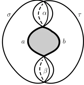
Areduction disc consists of a pair of distinct curves,↵, 2C( ,⌧), together
with arcs,a✓ andb✓⌧, connecting↵to , and with the same endpoints,
and such that a[b is homotopically trivial in M. (Figure 2)
We say that and ⌧ admit a reduction, if they admit a reductiion ball or
a reduction disc.
D B D0 ⌧
Figure 1. An example of a reduction ball. Note that and
⌧ might have other intersections.
↵
a b
⌧
Figure 2. An example of a reduction disc. Note that, again,
and⌧ might have other intersections, and that the homotopy
might not be embedded and might also intersect or ⌧.
As we explain in Section 4, this is easily seen to be equivalent to the notion of “normal position” as used in [HenOP] and [HilH] (generalising the notion of Hatcher [Hat]). We can therefore apply the results of those papers. In particular, the following is a consequence of Hatcher’s normal position:
Lemma 3.1. ,⌧ admit a realisation in normal position.
In fact, in view of Laudenbach’s theorem [L1], this can be achieved while
holding either or⌧ fixed. Again, this will be explained in Section 4.
Suppose that , 0 are in normal position. An innermost disc in 0 is an
embedded disc, D ✓ 0, such that @D = \D. Now @D cuts into two
discs, D1 and D2. Let ⌧i = D[Di. Thus, ⌧1,⌧2 are embedded essential
2-spheres inM. Pushing D slightly o↵ 0 on the side of the disc Di, we can
realise⌧i to be in general position with respect to 0. We can further pushDi
[image:10.612.232.377.263.410.2]to both⌧1 and⌧2 inS. We will say in this case that⌧i is obtained bysurgery
of along D. In practice it will be convenient in later constructions not to
carry out the second pushing operation. It will be sufficient to know that
and ⌧i are homotopically disjoint, without making them actually disjoint as
subsets of M. Therefore, when referring to a “surgery” henceforth we will
assume that we have pushed D, but not Di.
Definition. Given , 0 2V(S), we say that⌧ 2V(S) is obtained bysurgery
on in the direction of 0, if we can find realisations of , 0 in normal
position, and an innermost disc,D, in 0, such that⌧ 2{⌧1,⌧2}in the above
construction.
Note that, in general, one may need to homotope ⌧ further so that it is
in normal position with respect to 0 (but see Lemma 3.4 below).
Definition. Given , 0 2 V(S), a surgery path from to 0 is a sequence = 0, 1, . . . , n = 0 in V(S) such that for all i < n, i+1 is obtained by
surgery on i in the direction of 0.
Note that, if ⌧ is obtained by surgery on in the direction of 0, then
|C(⌧, 0)| < |C( , 0)|. From this, it is not hard to see that a surgery path
between two spheres and 0 always exists (see Lemma 3.4 or the discussion
in Section 4).
The following is proven in [HilH] (Theorem 1.2, thereof):
Theorem 3.2. [HilH] Surgery paths are uniform unparameterised quasi-geodesics.
Rather than recall the formal definitions, we just note here that (given
the hyperbolicity of S) this implies that any surgery path from to 0 is a
bounded Hausdor↵ distance from any geodesic inS from to 0, where the
bound depends only on g.
In this section, we will show:
Proposition 3.3. Let :S !S denote the map ◆ , and let 2V(S). For any 0 2 ( ), there is some surgery path, =
0, . . . , n= 0, from to 0 in S such that the diameter of Sn
i=0 ( i) in S is at most 16.
To see that this implies Theorem 1.2, let ⌧ 2 ⇧( ). (Recall that this
means that ⌧ 2 ◆A minimises dS( ,⌧) among all elements of ◆A). Given
that ◆A is (quasi)convex in S, it is easily seen, from the hyperbolicity of S,
that ⌧ lies a bounded distance from any geodesic from to any point of ◆A,
in particular 0. By Theorem 3.2, it follows that there is some i on the
surgery path given by Proposition 3.3 so that dS(⌧, i) is bounded. Since
by Proposition 3.3, diam({⌧}[ ( )) is also bounded. Theorem 1.2 now
follows on observing that ⇧( )3⌧ has bounded diameter.
The proof of Proposition 3.3 consists of several steps.
As a first step, Lemma 3.4 shows that, if we choose innermost discs appro-priately, there will be no need to homotope the spheres obtained in surgery in order to achieve normal position (that is, beyond pushing the innermost
disc slightly o↵ itself after doing the surgery).
Lemma 3.4. Let and 0 be two essential spheres inM in normal position.
Then there are at least two distinct innermost discs in 0, together with
spheres, obtained by surgering along each of these respective discs, which are in normal position with respect to 0.
Proof. We first make the elementary observation that surgery can never create any reduction discs.
Therefore, to make sure that a sphere obtained by surgering in the
direction of 0 is in normal position with respect to 0, we only need to
arrange that the surgery process does not create any reduction balls.
Now, define atube as a ball inM whose boundary has the formD[A[D0
where Dand D0 are innermost discs in 0 and A is an annulus in ; we also
allow the degenerate case where D = D0 and A is the boundary of D. We
call A the annular part of the tube.
We say that a tube T is contained in a tube T0 if the annular part of T is
contained in the annular part of T0. (This is equivalent to inclusion of the
respective balls.)
Now, let T be a tube which is maximal under containment. Write @T =
D[A[D0, as above. Let D1 ✓ be the disc with boundary @D, on the
opposite side ofA (or of D0 in the degenerate case). Then
1 =D[D1 is a
surgered sphere, which we push o↵ D so that it is in general position with
respect to 0. We write ˆD for the parallel copy of D. Let R ✓ M be the
ball with @R =D[AR[Dˆ, where AR✓ is an annulus.
We claim that 1 and 0 do not admit any reduction balls. The idea
is simple. If 1 and 0 admitted a reduction ball, then either and 0
admitted a reduction ball, or the tube T would not be maximal, leading to
a contradiction.
In fact, suppose two discs, E in 1 and E0 in 0 bound a reduction ball
B ✓ M. If the disc E does not contain ˆD, then E, E0 would also bound a
reduction ball for and 0, contradicting normal position of and 0. If E
does contain ˆD, then denote E\Dˆ by A0. Now, T \R = D, B \R = ˆD
D0[(A[AR[A0)[E0. It strictly contains T, contradicting the maximality
of T.
Hence 1 is in normal position with respect to 0. Similarly, D0 gives us
another sphere in normal position with respect to 0.
Note that, in the case of a degenerate tube, surgering on either side of
D=D0 yields spheres which are in normal position with respect to 0.
To conclude the proof, note that we always get at least two innermost
discs providing surgered spheres in normal position with respect to 0. In
fact, any non-degenerate tube will furnish two such discs, while if there are
only degenerate tubes, any two disjoint innermost discs in 0 will serve this
purpose. ⇤
As a next step, the aim of the following two lemmas is to show that, if
is a sphere inSand 0 is a sphere in ( ), then and 0 can be represented
simultaneously in normal position with respect to each other, and in efficient
position with respect to a map f : S ! M, in such a way that \f(S)
and 0 \f(S) are disjoint. This will be of fundamental importance in the
proof of Proposition 3.3.
Lemma 3.5. Suppose that , 0 are 2-spheres in M, and that f0 :S !M
is in general position, and efficient with respect to . Then there is a map
f homotopic to f0, efficient with respect to both and 0, and such that the
arcs of f 1( ) are homotopic to those of f 1 0 ( ).
Proof. Saying thatf0 is not efficient with respect to 0 is equivalent to saying
that there is an arc b in f0(@S) together with an arc c in 0 with the same
endpoints so that b[cis null homotopic in M; we will call such an arc b a
returning arc. We can assume that the arc cintersects each circle in \ 0
at most once (otherwise, we could just push it o↵ the disc bounded by this
circle). Now, let h : D ! M be a homotopy between the arcs b and c,
where D is a disc.
We claim that any arc in h 1( ) has one extremity on h 1(b) and the
other extremity on h 1(c).
By efficiency of f0 with respect to , no arc in h 1( ) can have both
extremities on h 1(b). Suppose there is an arc b0 in \h(D) having both
extremities onc. Letpandqbe its extremities. Since and 0 are in normal
position, the pointspand qlie on the same circle of \ 0, contradicting the
assumption that cintersects each circle in \ 0 at most once. This proves
the claim.
Now, construct a surface, S1, homeomorphic to S, by gluing D toS. We
do so by identifying the arcs h 1(b) ✓ @D and f 1
0 (b) ✓ @S via the map
f 1
S to S1. We define a map f1 = f0 [h : S [D ! M, map homotopic
to g (via the homotopy equivalence of S and S1). Moreover, the arcs in
f1 1( ) are homotopic to those of f0 1( ). By homotoping f0 tof1 we have
reduced the number of returning arcs. Continuing in the same way, we can
inductively eliminate all returning arcs and find a mapf :S !M efficient
with respect to 0, and such that the arcs of f 1( ) are homotopic to those
of f 1
0 ( ). ⇤
Lemma 3.6. Let be a sphere in S(M). For any sphere 0 in ( ), there
exist simultaneous realisations , 0 and f : S ! M, such that all the
following conditions hold:
(A1) and 0 are in normal position; (A2) f is efficient with respect to 0; (A3) f is efficient with respect to ; (A4) f 1( )\f 1( 0) =?.
Proof. Let be a sphere in S(M) and let f0 :S ! M be a map efficient
with respect to . Let a be an arc in f0 1( ) and let 0 be the sphere ◆(a).
Note that in this way we obtain all the spheres in ( ). Up to changing 0
by homotopy, we can suppose that 0 and are in normal position, i.e. they
satisfy (A1). For the rest of the proof, and 0 will remain fixed.
Now, the map f0 is efficient with respect to , but not necessarily with
respect to 0.
By Lemma 3.5, there is a map f homotopic to f0, efficient with respect
to 0, and such that the arcs of f 1( ) are homotopic to those of f 1
0 ( ).
This gives us properties (A2) and (A3).
To obtain (A4), note that, sincef is efficient with respect to 0, by Lemma
2.5, f 1( 0) contains only one arc, which is homotopic to the arc a (namely
that originally used to define the homotopy class of 0). We will simply
denote this arc by a.
It remains to remove any intersection points between f 1( ) andf 1( 0).
To this end, we define a2-gon inS as a disc whose boundary consists of a
pair of arcs in f 1( ) and f 1( 0) respectively. We refer to the intersection
points of these arcs as the vertices of the 2-gon. Similarly, we define a
3-gon in S, to be a disc whose boundary consists of a pair of arcs in f 1( )
and f 1( 0) (referred to as the internal sides) together with an arc in @S
(referred to as theboundary side). The intersection point of the two internal
sides is referred to as the vertex of the 3-gon.
Now by construction, no arc of f 1( ) can cross a; that is they are all
homotopically disjoint or equal to a. Moreover, all curves in f 1( ) and
f 1( ) andf 1( 0) are vertices of 2-gons or 3-gons. It is therefore sufficient
to eliminate these.
Let B be a 2-gon, with vertices p, q, with edges b ✓ f 1( ) and b0 ✓
f 1( 0). Since and 0 are in normal position, there are no reduction discs
between them. Therefore f(p) and f(q) have to lie on the same circle in
\ 0. Let C ✓ and C0 ✓ 0 be the discs bounded by , respectively
containing f(b) and f(b0). (Note that these arcs need not be embedded.)
LetGbe the abstract 2-sphere obtained by gluingC andC0 along , and let
✓ :G !M be the map which combines the inclusions ofC andC0. This is
locally injective, and it extends to a locally injective map,✓ :G⇥[ 1,1] !
M, where we identifyG⌘G⇥{0}. We can suppose that ✓ 1( )\✓ 1( 0)✓
G⇥{0}. Note that, f|@B factors through a map F : @B ! G, so that
f|@B =✓ F (where@B =b[b0). We can also assume thatf is transversal to
✓. In particular, we can find an annular neighbourhood,A✓S\@S, of@B,
and an extention,F :A !G⇥[ 1,1], of F with f|A=✓ F|A, and with
F(@A)✓G⇥{ 1,1}. Now ˆB =B[A✓S is a disc with@Bˆ ✓@A, and we
can suppose thatF(@Bˆ)✓G⇥{1}. Leth: ˆB !G⇥{1}by any continuous
map with h|@Bˆ =F|@Bˆ. Note that f|@Bˆ =✓ h|@Bˆ. We now modifyf by
replacing f|Bˆ by ✓ h. Note that we now have ˆB\f 1( )\f 1( 0) = ?
(since f( ˆB) \ \ 0 ✓ ✓(G ⇥ {1}) \ \ 0 = ?). We have therefore
reduced |f 1( ) \ f 1( 0)|. We can perturb f slightly to ensure that it
remains in general position. This surgery does not change the induced map of
fundamental groups, ⇡1(S) !⇡1(M). The new mapS !M is therefore
homotopic to the original. (The homotopy between them might not fix @S,
but this does not matter.)
Continuing in this manner, we eventually remove all 2-gons. Note that
we have not touchedf|@S in this process, so (A2) and (A3) remain valid.
Now any 3-gon can be eliminated simply by removing a small regular
neighbourhood of it in S. Given that there are now no 2-gons, any
com-ponent of f 1( ) or of f 1( 0) which crosses an internal edge of the 3-gon
must terminate on the boundary edge. It follows that this operation does
not change| \f(@S)|or| 0\f(@S)|, sof remains efficient. In other words,
(A2) and (A3) again remain valid. The process does not reintroduce any 2-gons, so continuing in this way, we eventually remove all 3-gons. This
finally achieves (A4). ⇤
The next lemma is aimed at showing that, while surgering towards 0,
we can keep spheres efficient with respect to a given map f :S !M.
Recall that an embedded curve, ✓ M, is efficient with respect to a
Lemma 3.7. Let be a sphere in M, let be an embedded curve, and let
D be a disc disjoint from with@D ⇢ . Suppose is efficient with respect to . Then is efficient with respect to both spheres obtained by surgering
along D.
Proof. Suppose is not efficient with repect to one of the spheres, 1,
ob-tained by surgery. Then there is a returning arc, a✓ , for 1. That is, its
endpoints lie in 1, and it is homotopic, inM, to to an arcb✓ 1. But now
b can be homotoped o↵ Din 1. It follows thata is also a returning arc for
, contradicting the fact that is efficient with respect to . ⇤
As an immediate consequence of Lemma 3.7, if is a sphere inM efficient
with respect to a map f : S ! M, and D is a disc disjoint from @S with
@D ✓ , then the two spheres obtained by surgering along D are both
efficient with respect tof :S !M.
We are now ready to prove the following:
Lemma 3.8. Let be a sphere in S, then for any 0 in ( ), there exists some surgery path, = 0, 1, . . . , n = 0, so that for each i the set ( i) contains a sphere homotopically disjoint from 0.
Proof. Let be a sphere in S, let h : S ! M be a map efficient with
respect to , let a be an arc in h 1( ) and let 0 be the sphere ◆(a). Note
that through the process we just described we can obtain any sphere in ( ).
Let f : S !M be a map so that , 0, and f satisfy conditions (A1)–
(A4) of Lemma 3.6. For the rest of the proof, f :S !M, and 0 will be
fixed.
Now, f is efficient with respect to 0, and therefore, by Lemma 2.5,
f 1( 0) contains exactly one arc, call it a0, homotopic to a, and possibly
some inessential closed curves. Denote f(a0) by ✓ 0.
By property (A4) in Lemma 3.6, is disjoint from . This implies that
is contained in at most one innermost disc of 0. Hence, by Lemma 3.4,
there exist an innermost disc D in 0 disjoint from f(@S), and a sphere
1 obtained by surgering along D, so that 1 is in normal position with
respect to 0. (Recall we have pushed the discDslightly o↵ itself in forming
1.)
Now, since D is disjoint from f(@S), by Lemma 3.7 the sphere 1 is also
efficient with respect tof.
By construction and since the disc D is disjoint from f(@S), each arc in
f 1(
1) is, up to homotopy, also contained inf 1( ). This means that any
arc in f 1(
1) is at distance at most 1 in A from the arc a. Consequently,
by efficiency of 1 with respect to f, the projection of 1 contains a sphere
Now consider the spheres 1 and 0. They are in normal position with
respect to each other, the mapf :S !M is efficient with respect to both
spheres, and moreover, f(S)\ 1 is disjoint from f(S)\ 0 (since f(S)\
is disjoint from f(S)\ 0 and
1\ 0 is contained in \ 0).
Summarising, 1, 0 and f : S ! M also satisfy conditions (A1)–(A4)
of Lemma 3.6.
Therefore, using the same argument as above, we can find an innermost
disc D0 in 0 disjoint fromf(@S), and a sphere
2, obtained by surgering 1
along D0, in normal position with respect to
1, and efficient with respect
to f. By construction arcs in f 1(
2) are contained, up to homotopy, in
f 1(
1) and therefore are homotopically disjoint from a, consequently the
projection of 2 contains a sphere homotopically disjoint from 0.
As above one can check that 2, 0 andf :S !M satisfy the conditions
of Lemma 3.6.
We proceed inductively in this way, until we obtain a sphere n 1 which
is disjoint from 0.
The path , 1, 2, . . . , n 1, n = 0 is a surgery path satisfying the
de-sired property. ⇤
Proposition 3.3 immediately follows from Lemma 3.8, having noticed that is defined up to distance 7.
This completes the proof of Theorem 1.2.
4. Equivalence between definitions of normal position
In this section, we briefly review the notion of “normal position” for two 2-spheres in a 3-manifold, which was used in Section 3. Here we only
con-sider the case where the 3-manifold,M, is a doubled handlebody. (A similar
discussion would apply to a general compact 3-manifold, by taking the con-nected sum decomposition into irreducible components.)
First recall that Hatcher defined a notion of “normal form” for a system of disjoint spheres with respect to a maximal sphere system. In [HenOP] this was generalised to non-maximal systems. This gives a more symmetric notion. Their notion is used for the surgery construction in [HilH]. Other discussions of this notion can be found in [GP] and [I]. Here, for simplicity of exposition, we only consider the intersection of two spheres (though the arguments readily adapt to two sphere systems).
Let ,⌧ ✓ M be embedded 2-spheres in general position. Lemma 7.2 of
Definition. ,⌧ are innormal position if
(N1) each lift of to the universal cover, ˜M, meets each lift of⌧ in at most
one curve, and
(N2) no complementary component of the union of two such lifts is a ball in ˜
M.
It is easy to see that this is equivalent to saying that and 0 do not
admit any reductions, hence to saying that they are in “normal position” as we defined it in Section 3. In fact, condition (N1) (respectively condition
(N2)) is equivalent to saying that and ⌧ do not admit any reduction discs
(respectively any reduction balls).
As noted in Section 3 (Lemma 3.1), a normal position for two spheres
and ⌧ always exists. This is a straightforward consequence of Proposition
1.1 of [Hat] and Lemma 7.2 in [HenOP].
Indeed, normal position is equivalent to minimal intersection of two spheres. This can be deduced from the discussion in [GP]. However, for the sake of completeness, we give below another proof.
To clarify terminology, recall that C( ,⌧) is the set of components of
\⌧. Let ( ,⌧) be the minimum of |C( ,⌧)|, as and ⌧ vary over their
respective homotopy classes. Note that, in view of Laudenbach’s theorem,
in order to define ( ,⌧), we could hold fixed, and just allow ⌧ to vary in
its homotopy class.
Lemma 4.1. ,⌧ are in normal position if and only if |C( ,⌧)|=( ,⌧).
Proof. We first observe that if there are no innermost reduction balls, then there are no reduction balls at all. Moreover, we can always surger out any
innermost reduction ball and reduce|C( ,⌧)|. We can therefore assume that
there are never any reduction balls.
To conclude the proof, we lift to the universal cover ˜M. (This is a
3-sphere minus an unknotted Cantor set.) Let s ✓ M˜ be any component of
the lift of , which, as noted above, we can assume to be fixed. Let T(⌧)
be the set of lifts of ⌧, and let T0(⌧) = {t 2 T(⌧) | t\s 6= ?}. Note that
|T0(⌧)||C( ,⌧)|, with equality if and only if there are no reduction discs.
Suppose first, that there are no reduction discs. In this case, we see that
if t2T0(⌧), thent0\s6=?for any 2-sphere, t0, homotopic to t in ˜M. (This
follows since the sets of ends of ˜M separated bys andtare non-nested: they
pairwise intersect in four non-empty sets. But these sets do not change on
replacing t by t0.) In particular, if ⌧0 is homotopic to ⌧ inM, then
Therefore, ⌧ minimises |C( ,⌧)|. In other words, ( ,⌧) = C( ,⌧). This shows that normal position implies minimality.
Conversely, suppose that ,⌧0satisfy|C( ,⌧0)|=( ,⌧0). Now, by Lemma
3.1, we can certainly choose⌧ so that and⌧ admit no reductions. But now,
the above inequality must be an equality. In particular,|T0(⌧0)|=|C( ,⌧0)|,
so and ⌧0 do not admit any reductions either. ⇤
References
[AS] J.Aramayona, J.Souto,Automorphisms of the graph of free splittings : Michigan Math. J.60(2011) 483–493.
[F] M.Forlini,Splittings of free groups from arcs and curves: preprint (2015), posted at arXiv:1511.09446.
[GP] S.Gadgil, S.Pandit,Algebraic and geometric intersection numbers for free groups : Topology Appl.156(2009) 1615–1619.
[HamH] U.Hamenst¨adt, S.Hensel, Spheres and projections for Out(Fn) : J. Topol. 8
(2015) 65–92.
[HanM] M.Handel, L.Mosher,The free splitting complex of a free group, I: hyperbolicity : Geom. Topol.17 (2013) 1581–1672.
[Hat] A.Hatcher,Homological stability for automorphism groups of free groups: Com-ment. Math. Helv.70(1995) 39–62.
[Hem] J.Hempel,3-manifolds: Annals of Mathematics Studies No. 86, Princeton Uni-versity Press (1976).
[HenOP] S.Hensel, D.Osajda, P.Przytycki, Realisation and dismantlability : Geom. Topol.18(2014) 2079–2126.
[HenPW] S.Hensel, P.Przytycki, R.Webb,1-slim triangles and uniform hyperbolicity for arc graphs and curve graphs : J. Eur. Math. Soc.17(2015) 755–762.
[HilH] A.Hilion, C.Horbez,The hyperbolicity of the sphere complex via surgery paths : to appear in J. Reine Angew. Math.
[Hir] M.W.Hirch, Di↵erential topology : Graduate Texts in Mathematics, Springer-Verlag (1976).
[I] F.Iezzi,Sphere systems in 3-manifolds and arc graphs : PhD thesis, University of Warwick (2016), available at http://wrap.warwick.ac.uk/78841/
[L1] F.Laudenbach,Sur les 2-sph`eres d’une vari´et´e de dimension3 : Ann. of Math.
97(1973) 57–81.
[L2] F.Laudenbach, Topologie de la dimension trois: homotopie et isotopie : Ast´erisque No. 12, Soci´et´e Math´ematique de France, Paris (1974).
[MS] H.Masur, S.SchleimerThe geometry of the disk complex : J. Amer. Math. Soc.
26(2013) 1–62.