HANDBOOK OF
ANALOG
HANDBOOK OF
ANALOG
NOTICE
In order to enable us to process your requests for spare parts and replacement items quickly and efficiently, we request your conformance with the following procedure:
1. Please specify the type number and serial number of the basic unit as well as the EAI part number and de-scription of the part when inquiring about replacement items such as potentiometer assemblies or cups, re-lays, transformers, precision resistors, etc. 2. When inquiring about items as servo multipliers,
re-solvers, networks, printed circuit assemblies, etc., please specify the serial numbers of the major equip-ment with which the units are to be used, such as: Console, Type 8811, Memory Module, Type 4.204, Serial No. 000, etc. If at all possible, please in-clude the purchase order or the EAI project number under which the equipment was originally procured.
Your cooperation in supplying the required information will speed the proceSSing of your requests and aid in assuring that the correct items are supplied.
It is the policy of Electronic Associates, Inc. to supply equipment patterned as closely as possi-ble to the requirements of the individual customer. This is accomplished, without incurring the prohibitive costs of custom design, by substituting new components, modifying standard com-ponents, etc., wherever necessary to expedite conformance with requirements. As a result, this instruction manual, which has been written to cover standard equipment, may not entirely concur in its content with the equipment supplied. It is felt, however, that a technically quali-fied person will find the manual a fully adequate guide in understanding, operating, and
main-taining the equipment actually supplied.
ELECTRONIC ASSOCIATES, INC.
UNITED STATES AND CANADIAN OPERATIONS
Eastern United States
Southeast United States
Central United States
Southern United States
Western United States
LOCATION
West Long Branch, New Jersey
185 Monmouth Parkway West Long Branch, N.J. 07764 TWX: 710-722-6597 TELEX: 132-443
CABLE: PACE W. Long Branch, N.J. TELE: 201229-1100
Long Branch, New Jersey
Long Branch & Naberal Ave. Long Branch, N.J. 07740 TELE: 201229-4400
CABLE: PACE W. Long Branch, N.J.
Princeton, New Jersey u.s. Route No.1 P.O. Box 582 Princeton, N.J. 08541 TELE: 609452-2900
Dedham, Massachusetts
875 Providence Highway Dedham, Massachusetts 02026 TELE: 617326-6756
Rockville, Maryland
12260Wilkins Avenue Rockville, Maryland 20852 TELE: 301933-4100
Orlando District Office
7040 Lake Ellenor Drive Orlando, Florida 32809 TELE: 305851-0640
Des Plaines, Illinois
3166 Des Plaines Avenue Des Plaines, Illinois 60018 TELE: 312296-8171
Cleveland, Ohio
6500 Pearl Road Cleveland, Ohio 44130 TELE: 216884-4406
Dallas, Texas
3514 Cedar Springs Road Room 211
Dallas, Texas 75219 TELE: 214528-4920
Houston, Texas
7007 Gulf Freeway Room 128 Houston, Texas 77017 TE LE: 713 644-3678
Huntsville, Alabama
P.o. Box 4108 1000 Airport Road Suite F-2
Huntsville, Alabama 35802 TELE: 205881-7031
EI Segundo, California
1500 East Imperial Highway EI Segundo, California 90245 TELE: 213322-3124 TWX: 910-348-6284
Denver, Colorado
2120 S. Ash St. Denver, Colorado 80222 TELE: 303757-8341
FACILITIES
Corporate Headquarters Computer Division Computer Service Division
Principal Engineering and Manufacturing Sales and Service
I nternational Operations
Graphics and Instrument Division G & I Engineering and Manufacturing
Computation Center, Education & Training
Sales and Service
Sales and Service Computation Center
Sales and Service
Sales and Service
Sales and Service
Sales and Service
Sales and Service
Sales and Service
Sales and Service Computation Center
Canada
United Kingdom
Sweden
European Continent
France
Germany
Australia & New Zealand
Australia & New Zealand
Japan
Mexico
LOCATION Seattle, Washington
1107 N.E. 45th St., Room 323 Seattle, Washington 98105 TELE: 206632·7470
Palo Alto, California
4151 Middlefield Road Palo Alto, California 94303 TELE: 415321·0363 TWX: 910-373·1241 TELE: 415·321·7801*
Allan Crawford Associates, Ltd.
65 Martin Ross Avenue Downsview, Ontario, Canada TELE: 416636-4910
FACILITIES
Sales and Service
Sales and Service Computation Center *Scientific Instrument Division
Engineering and Manufacturing
Sales and Service
INTERNATIONAL OPERATIONS
LOCATION
Electronic Associates, Ltd.
Victoria Road
Burgess Hill, Sussex, England TELE: Burgess Hill (Sussex)
5101-10,5201·5 TELEX: 851·87183 CABLE: PACE Burgess Hill
Northern Area Office
Roberts House Manchester Road Altrincham, Cheshire TELE: Altrincham 5426
FACILITIES
Sales and Service
Engineering and Manufacturing Computation Center
Sales and Service
EAI Electronic Associates-AB: Hagavagen 14
Solna 3, Sweden TELE: Stockholm 82-40-97 TE LEX: Stockholm 854-10064 CABLE: PACE STOCKHOLM
Electronic Associates, Inc.
116·120 rue des Palais Brussels-3, Belgium TELE: 16.81.15 TELEX: 846·21106 CABLE: PACEBELG Brussels
EAI-Electronic Associates SAR L
72-74 rue de la Tombe Issoire Paris 14e, France TE LE: 535.01.07 TELEX: 842-27610
EAI-Electronic Associates GMBH
5100Aachen, Bergdriesch 37, W. Germany
.TELE: Aachen 2 6042: 26041 TELEX: 841·832676 eaid
EAI-Electronic Associates, Pty. Ltd.
26 Albany Street
St. Leonards,-N.S.W. Australia TE LE: 43·7522 (4 lines) CABLE: PACEAUS, Sydney
Victorian Office
11 Chester Street
Oak leigh Victoria, Australia 3166 TELE: 569·0961 569·0962 CABLE: PACEAUS, Melbourne
Sales and Service
Sales and Service
Sales and Service
Sales and Service
Sales and Service
Sales and Service
EAI-Electronic Associates, (Japan) Inc. Sales and Service 1·3 Shiba·Atago·cho
Minato-ku Tokyo, Japan 105 TELE: 433-4671 TELEX: 781-4285 CABLE: EAIJAPACE
HANDBOOK OF ANALOG COMPUTATION
Prepared by
The Education and Training Department
Edited by
Alan Carlson, George Hannauer,
Thomas Carey and Peter J. Holsberg
SECOND EDITION
Electronic Associates, Inc.
Princeton, New Jersey
~ Electronic Associates, Inc., 1967 -- All Rights Reserved
PREFACE
These notes on Analog Simulation have been developed from the experience
gained by the Education and Training Department of EAI in presenting intensive short courses in analog computer operation, programming, and applications for nearly a decade.
The objective of these courses has been to provide scientists and enginee~s
with a working knowledge of the analog computer and its uses. They have
pro-ven to be most effective when lectures and demonstrations are supplemented with
laboratory sessions allowing students to put theory into practice. The
solu-tion of problems on an analog computer, using effective and efficient program-ming techniques and check-out procedures, has proven to be invaluable in gaining familiarity both with the machine and its potential as an engineering tool.
Many of the procedures and techniques described in the notes have been used and found to be effective in EAI Computation Centers throughout the world.
A course in analog computation utilizing these notes could readily meet the requirements of an accredited, one semester, 3-credit-hour university course. A course in differential equations as a prerequisite is desirable.
The wide range of application for the analog computer permits the introduc-tion of actual applicaintroduc-tions appropriate to courses in all scientific disci-plines. The EAI Applications Reference Library is a source of a large number of such studies describing applications in such areas as electronics, chemical processing, aerospace engineering, and life sciences.
These notes represent the combined efforts of a large number of people within
the EAI organization. Contribution to the notes and the editing were made by
A. I. Katz, O. Serlin, H. Davidson, and J. J. Kennedy, as well as many others.
Many sections in the notes were derived from material generated by the various Departments in the Research and Computation Division of EAI.
TABLE OF CONTENTS
CHAPTER I ••••• THE ANALOG COMPUTER AND ITS ROLE IN ENGINEERING ANALYSIS. • • . 1
CHAPTER II.oooTHE GENERAL PURPOSE ANALOG COMPUTER . . . 0 • • • • 16
CHAPTER 1110 • • ANALOG COMPUTER PROGRAMMING AND CHECKING PROCEDURES . . . .84
CHAPTER IV.oo.ANALYSIS OF LINEAR AND NON-LINEAR SYSTEMS 0 • 0 • • • • • • • 135
CHAPTER Vo •••• TECHNIQUES IN FUNCTION GENERATION • . 0 • • • • 0 • • 0 0 • • 163
CHAPTER Vloo •• TRANSFER FUNCTION SIMULATION . . . 0 0 • • • • 0 • • 0 0 • • • 191
CHAPTER VII. 0 • TRANSPORT DELAY SIMULATION 0 0 0 0 • • • 0 • It • . • • • • • • • 220
CHAPTER VIII •• REPETITlVE OPERATION. 0 • • • • • • • 0 • 0 • • 0 • 0 • • • • 241
CHAPTER IX 0 o •• ANALOG MEMORY . . . 0 • • • • • • • • • • • • • • • • • • 248
CHAPTER X ••••• PROBLEM PREPARATION PROCEDURE • . 0 • 0 • • 0 • • • • • • • • 260
CHAPTER XI ••• o ANALOG COMPUTER SOLUTION OF PARTIAL DIFFERENTIAL EQUATIONS . 279
CHAPTER XII ••• ACCURACY OF ANALOG COMPUTER SOLUTIONS 0 • 0 • • • 0 • • • • • 289
CHAPTER XIII •• EXAMPLES OF EFFICIENT PROGRAMMING . . . 0 ~ • • • • • • • • • 296
CHAPTER XIV ••. FACTORS IN PLANNING AND OPERATING AN ANALOG LABORATORY . • . 354
Appendix Ao.~.LaPlace Transforms . . • 0 • • • 0 0 • • 0 • • • • • • • • • • 366
Appendix B.o •• Transfer Function Circuits. 369
Appendix C.o •. Diode and Relay Circuits. 375
CHAPTER I
THE ANALOG COMPUTER AND ITS ROLE IN ENGINEERING ANALYSIS
A. Introduction
The role of the electronic, general purpose analog computer in modern-day industry best can be explained by considering the concept of engineering de-sign. When a design is required, one or more engineers or scientists propose a system which they feel 'viIi satisfy the design criteria. Design proposals, however, involve approximations and estimates and there may not be concrete agreement as to which design is best. Therefore, some form of evaluation of the proposed system is desirable.
In evaluating proposed systems or designs, one can, in general, select either of two paths: an experimental program, or an analytical evaluation of the system. The experimental approach is usually characterized by a minimum of of analysis, the construction of a prototype of the system, and considerable "trial-and-error" experimental work. The objectives are to evaluate the experi-mental data and suggest appropriate modifications which will result eventually in an optimum or nearly optimum design. The cost and time required for this experimental approach are normally much greater than those incurred in an analytical evaluation. In the analytical approach,the task is to derive a set of equations (a mathematical model) whose solution will describe the behavior of the system in terms of its geometry, time, and parameters. These solutions then can be used to obtain operating conditions and parameters which will re-sult in optimum system performance.
Since the derivation of mathematical models frequently requires approximations, and the results obtained are often based on limited input data, prototype
experimentation usually is required. However, pilot plants designed on the basis of extensive analytical investigations frequently are near optimum and
require little or no modification. The only experimenta~esults required
are those which validate the mathematical model. Once the model is validated, additional experimentation can be performed analytically, which results in a considerable cost reduction compared 'to the experimental approach.
Not all proposed designs, unfortunately, lend themselves to a choice of evalua-tion programs. If one cannot obtain a mathematical model, there is no recourse except an experimental program. On the other hand, if the cost of a prototyp~
is prohibitive (e.g. a nuclear reactor),its design is restricted to analysis. The major considerations in selecting the proper evaluation path are a compro-mise between cost, time, and objectives.
B. Ma thema ti ca 1 M()'de 1 s
The analyst then can derive equations for each subsystem, and the set of
equa-tions is the mathematical model for the entire system. The individual
equa-tions are derived from basic mathematics and physical laws such as the conser-vation of energy, matter, etc. and, at times, from empirical and semi-empirical
equations such as fluid film resistance in heat transfer. The mathematical
model can be a collection of integral or algebraic equations, although differ-ential equations are most frequently obtained.
Typical examples Jf equations encountered in practical applications are:
1) Algebraic and Transcendental Equations, e.g. the effect of
temper~ture on physi~a1 properties of materials. Thus
k
=
thermal conductivity of a metal=
k+
aTo
Cp
=
specific heat of a gas a+
bT+
cT2-A T
~
=
viscosity of a fluid=
~ eo
2) Ordinary Differential Equations, e.g. the kinetics of a chemical
reaction
A 2B
x
whose mathematical model is
and
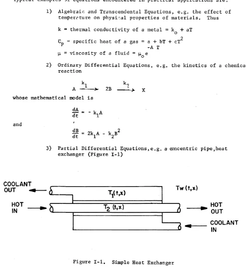
COOLANT
OUT
~HOT
IN
dA
= - k A
dt 1
3) Partial Differential Equations,e.g. a amcentric pipe,heat exchanger (Figure I-I)
h
T
t
(
f ,x)Tw
(f,x)•
HOT
~h
T2
(ftx) ~OUT
I
COOLANT
6
4 [image:10.613.52.546.188.739.2]IN
whose mathematical model is
oT
2 ~T2.
+
a2 (T2 - Tw) 0
~ + V2 ox
where
T (t,x) wall temperature
w
Tl (t,x) coolant temperature
T
2(t,x) primary (hot) fluid temperature
Two types of models, linear or nonlinear, are possible and are a
measure of the complexity of the system. Simple linear models are "nicer"
since they lend themselves to rapid analytical solutions. Unfortunately,
be-cause of the interaction of physical laws, the need for semi-empirical or em-pirical equations to des~ribe this interaction, and the nature of most physical systems themselves, the majority of the mathematical models encountered in practice are nonlinear. This is unfortunate because little is known about the analytical solutions to nonlinear equations, and those solutions that are obtained are usually difficult to interpret and evaluate. If a system is nonlinear, its behavior is a function of its initial conditions, which makes its analysis even more essential if optimum performance is desired.
C. Solving Mathematical Models
Solutions of mathematical models can be obtained analytically by classical methods, numerical methods, or by electronic computation.
Classical solutions of simple models are possible if the model is composed of ordinary linear and/or partial differential equations and certain classes of
non-linear differential equations. Frequently, this technique can be applied
Numerical solutions involve the transformation of a mathematical model into a set of algebraic equations by replacing all derivatives in the model with
appropriate algebraic, finite difference approximations. The resultant set
of algebraic equations is then solved simultaneously to affect a solution. This technique not only is time consuming but may suffer from accuracy, sta-bility and convergence problems.
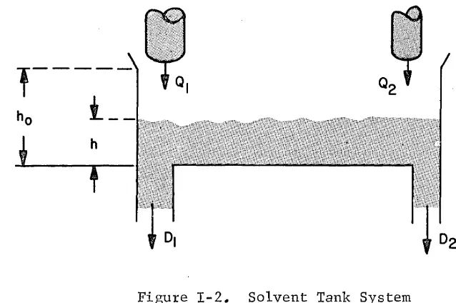
To illustrate the classical and numerical solutions for a differential equa-tion, consider the problem of a solvent tank (Figure 1-2) which can be filled
by two feed streams (Ql and Q2) in 4 and 5 hours respectively. Two drain
pipes, Dl and D 2,
Figure 1-2. Solvent Tank System
can empty the tank in 3md 6 hours respectively. If the tank is half full
and all feed and effluent streams are used will the tank fill, empty, or reach steady-state? How long will it take?
The mathematical model for the tank is the nonlinear differential equation
~
dt (1)
where
y hlh
a (2)
[image:12.617.76.395.202.414.2]Y dy
v;-I
1:J
2f!,dl.l c:t0.45-y2 v;:0.45-1-L
Yo=~ ~o= ~
(3)
or,
0.9 ln 0.45 0.45
-~
-\fY
+
2([; 2--{4;)
y = t (4)The obvious difficulty in applying this equation is that y, the level in the tank, does not appear as an explicit function of time, t. Even though we have an analytical solution, considerable effort is still required to produce a
useful relation between y and t, say, in the form of a graph. The eventual
height of the solvent in the tank will be the steady-state solution, y , of
e~ation (1) ( obtainedby letting dy/dt equal zero) s
y = (0.45)2 = 0.203
s (5)
The time required to reach this height in theory is infinite; therefore, a practical value of the steady state time must be obtained graphically from a plot of y versus t.
Since the time required to attain the equilibrium height also can be obtained
from a numerical solution of equation
(U,
let us now consider this method ofsolution.
Integrating equation (1) one obtains
t
y 0.45 t
-f
Yo
1: 2
dt +y
o (6)
where the initial value of y, y is 0.500. Recalling that integration is
the area under a curve, Figure £-3, equation (6) can be rewritten in terms
of finite or discrete intervals of time:
where
= y
+
0.45 nf::. to
t
=
n f::. tn=co
-I
f::.t (7)n=l
(8)
The accuracy of the solution obtained from this equation depends on the
FUNCTION OF TIME
0.450
'IIII~=~
__
O~
tt, t2
INTEGRAL OF THE FUNCTION
Y 1:
2
o
Ij~I!1 ~~~eE
UNDER•
ERROR DUE TO
FINITE APPROXIMATION OF INTEGRAL
---I!I
...
t--~~~---~·t
Equation (7) is solved in the fol.lm~li ng ,~:rrrrr::" :~:t dEtra:r :.~L 0.~E' c';::~n sele;;.:tecl;
at say
0.5
hours.1) Compute Y"2
n -1
2)
3)
4)
5)
6)
Compute
Compute
Compute
Compute
Let n
--0.45
Yn
n
+
(Yo ia known and LS U5~: ~s G startj~3 point)
n~t
1 and retut'n to f;tep 1.
Results obtained from both the numerical and .. m.ulytical solutio:ns are shown
in Figure 1-4.
y:JL ho
0.5 t
o NUHERICAL RESULTS
o
ANALYTICAL RESULTS0.4
0.3
o
0.2
--1----_ _ _ _ _ _
-=::::~==~==:il=~ddo
2 3 4 4.5
TIME IN HOURS
From the curve shown in Figure 1-4, it is apparent that the tank (Figure 1-2)
will fill and reach equilibrium in approximately 4.5 hours. It should be noted
that an increase in the accuracy of the numerical solution would have required
additional computations and, hence, increased computation time. The same
procedure would have been followed for a smaller increment of time, ~t. The
error of the numerical solution is indicated by comparison to analytical
re-sults obtained from equation (4). Computer solutions are best understood
after an explanation of the type and methods of computer operation is
pre-sented. However, it is convenient to point out at this time that the
numeri-cal solution illustrated above is typinumeri-cal of digital computer solutions and the itemized instructions are typical of a digital computer flow chart.
If one considers a flow diagram for the solution of equation (6), which is shown in Figure 1-5, insight to the analog computer solution can be obtained. It will be shown later that the analog computer is composed of components which perform the mathematical operations described in Figure 1-5.
f
0.45
-
}:
Oo4s!dt
-_.
L
y (t )Yo
-
--
-tY I /2( t)
[:t
-h
l/2dt
..
-y"2{t)
V-
--e 1-5: Flow Diagram of Solv--ent Tank Figur
Solution
At this point, the justification for using computers can be considered.
In our modern society, machinery of various sorts has relieved human muscle
from a great deal of routine and repetitive operation. In doing so, it has
multiplied the effectiveness of that human muscle both in industry and in the home.
The computer has performed a similar service for the mind essentially by mechanizing routine mental processes, leaving the mind free to examine new
problem areas. Studies of the behavior of entire complex systems can ,be
performed with great speed and, consequently, our actual knowledge of complex
systems has increased greatly. Equally important, our capacity for control and
prediction, and for insight into these complex systems also has been extended. The inf~uence of the computer on our common life, therefore, lies in its con-tribution, in the broadest sense, to science and technology.
Investigations in science and engineering can be carried out on a scale
un-heard of only one or two decades ago. Scientific principles and models can
considerable flexibility. Thus, new areas of scientific knowledge have been established and will continue to grow as a result of research and development performed on computers.
D. Computer History and Characteristics
A computer is a device that is able to receive information (equations, instruc-tions, data, etc.) and process it in a predetermined manner to obtain useable results.
For example, a human being may be a computer. He can take information in
through his senses, use principles stored in his memory to process or perform operations on this information in many ways, and produce an answer, perhaps in the form of an action.
Similarly, a machine may be able to accept information of a suitable form, receive instructions on how to operate on this information, perform the re-quired operations, and give the answers. Machines may take many forms vary-ing from simple beads on a frame to the incredibly complex, expensive and highly sophisticated modern machines.
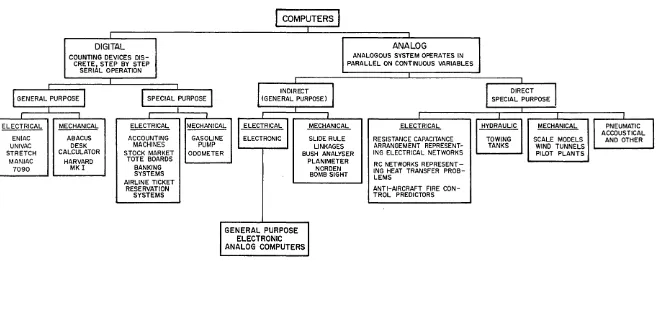
1. Early Computers---The history of computing devices may well extend to the
very beginning of civilization. For our purposes, they can be divided into
two categories (see Figure I-6):
o Mathematical instruments, the more complex of which are known
as analog computers. These are exemplified in simple form by
the slide rule.
o Calculating machines, more often known as digital computers. These can be represented simply by the desk calculator.
Early forms of digital computations could be considered to exist when man first started to use his fingers or pebbles for counting.
The earliest known record of analog computation is its use in surveying and
map making for the purpose of taxation (Babylonia, 3800 Be). The earliest
digital machine is probably the Abacus. In its early form, it consisted of
a clay board with grooves in which pebbles were placed. It later appeared
in the form of a wire frame with beads. It is still used extensively in Asia
and the East for remarkably rapid calculations.
The development of computational aids can be traced from these early instru-ments through the invention of logarithms, slide rules, linkages, analytical engines, and desk calculators to the large-scale general-purpose machines of the present day.
The first large-scale general-purpose digital computer was completed at Harvard
in 1944. This machine, the Harvard MBrk I Calculator, was built jointly by
IBM and Harvard, and used electromechanical relays. The Moore School of
I I-'
o
I
1
COMPUTERSI
I
DIGITAL ANALOG
COUNTING DEVICES DIS- ANALOGOUS SYSTEM OPERATES IN
CRETE,STEP BY STEP PARALLEL ON CONTINUOUS VARIABLES
SERIAL OPERATION
i
I
~ INDIRECT
I
l
GENERAL PURPOSEI
I
SPECIAL PURPOSEI
(GENERAL PURPOSE)I I
I I _I i I
ELECTRICAL MECHANICAL ELECTRICAL MECHANICAL ELECTRICAL MECHANICAL ELECTRICAL
ENIAC ABACUS ACCOUNTING GASOLINE ELECTRONIC SLIDE RULE RESISTANCE CAPACITANCE
UNIVAC DESK MACHINES PUMP LINKAGES ARRANGEMENT
REPRESENT-STRETCH CALCULATOR STOCK MARKET ODOMETER BUSH ANALYSER ING ELECTRICAL NETWORKS
MANIAC HARVARD TOTE BOARDS PLANIMETER R C NETWORKS
REPRESENT-7090 MKI BANKING NORDEN ING HEAT TRANSFER
PROB-SYSTEMS BOMB SIGHT LEMS
AIRLINE TICKET
RESERVATION ANTI-AIRCRAFT FIRE
CON-SYSTEMS TROL PREDICTORS
GENERAL PURPOSE ELECTRONIC ANALOG COMPUTERS
Figure 1-6 Computer Devices
I
DIRECTI
SPECIAL PURPOSE
J -.l i
HYDRAULIC MECHANICAL PNEUMATIC ACCOUSTICAL TOWING SCALE MODELS AND OTHER
[image:18.793.82.738.161.486.2]Proving Grounds in 1944. This machine, the
ENIAC,
~hich contained 18000 vacuum tubes, now has many direct descendents.Mechanical integrating devices of the late 19th century were improved on during World War I, when Hannibal Ford increased the torque output of the ball-and-disc integrator and used it to make a naval gun fire computer. This was followed by more experimentation in the 1920's.
At M.I.To, Dr. Vannevar Bush completed the first large-scale mechanical
differential analyzer in 1931. This machine is now installed at Wayne
University in Detroit where it is still being used effectively. At the present time, there are several large scale mechanical machines in
opera-tion. Simultaneous equation solvers and harmonic analyzers of many types
also appeared in the 1930's.
Special computers, in the form of network analyzers for the simulation of
power networks, appeared around 1925. The network analyzer is a passive
element analog. A scale model of the particular network to be studied is made with resistors, capacitors, etc. The early network analyzers could be used
to investigate only steady state problems; that is, voltage drops along
lines, possible current flow in lines, etc. The most recent network analyzers can be used to investigate transient conditions during faults on networks or
switching on networks. These may be considered to be true general-purpose
computers.
2. Analog and Digital Computers---In digital computers, numbers are
oper-ated upon directly. The basic operation in these machines is counting. This
enables the machine to perform the four fundamental operations of arithmetic,
addition, subtraction, multiplication and division. The basic operation of
any digital computer is similar to that of the abacus where numbers are repre-sented by.beads and the counting of these beads is the basis of addition and subtraction. In digital computers, all mathematical calculations depend ul-timately on counting, whether it be beads, gear teeth, or electrical pulses.
In analog machines, numbers are reoresented by physical quantities whose
magnitude is determined by the magnitude of the number. Mathematical
operations are represented by physical events; that is, the machines do not count, but perform continuous manipulations equivalent to the mathematical
operation required. The result of these manipulations is another physical
quantity, whose magnitude and behavior represents the solution to the pro-blem.
Probably the most useful example of the analog computer is the slide rule. Here, to multiply one number by another, the discrete numbers are converted
to logarithms, the logarithms are converted to linear distances on sticks which, when placed end to end (i.e. added together--the continuous operation
There exists on the analog a complete analogy between the physical quantities,
events, and the mathematical numbers and manipulations. If many events are
taking place at the same time in the physical world, they will also take place
at the same time, or in parallel, on the machine. An analog device will,
con-sequently, arrive at a result in a shorter time than a digital machine which must perform all its operations serially.
The precision of a digital machine is theoretically boundless. To increase by
ten the precision of a decimal counting device, it is a matter simply of
accomo-dating one more place (decimal) throughout the equipment. However, to achieve
the same end on the analog, e.g. the slide rule, the length of the slide rule
would have to increase by a factor of ten. This is not always practicable.
Analog devices, are characterized by continuous operations performed in parallel,
as opposed to digita.l machines which are discrete, 'serial devices. The analog
solutions are obtained in a continuous manner since all parts of these devices operate simultaneously.
3. General Purpose Analog Computers---We have said that in analog devices
numbers are represented by physical quantities. Theoretically, any physical
quantity may be used as long as it can be made to obey those laws necessary to represent the mathematical relationships involved in the original problem. Purely electrical relationships, which have the mechanical advantage of no moving parts and, a high speed of operation, have been found most suitable
for analog devices.
The introduction of the operational amplifier made possible the newest class of general purpose analog computers using voltages as the 'physical quantity' .
Lovell of Bell Telephone Laboratories is generally credited with the
introduc-tion of the operaintroduc-tional amplifier during the Second World War. These
ampli-fiers can be divided into two groups, those which op~rate on a-c voltages and
those which operate on d-c voltages. The a-c amplifiers exhibit certain
dif-ficulties and do not lend themselves to any direct form of integration. Therefore,only d-c amplifiers are considered in these notes since they are
most common in comrner~ially available general purpose analog computers.
E. Industrial Uses of the Analog Computer
As a result of the tremendous competition in industry following World War II,
more economical designs and more thorough evaluations were needed. The
con-cept of a fully automated plant, or system, operating at an economic optimum, demanded from the engineer a more extensive knowledge of each element, and
its behavior. The engineers, in turn, demanded a more complete analysis of
mechanisms and transport properties from the basic research scientists.
1. Initial Research and Development---The initial work in development
usually takes place in the laboratory where bench-scale studies, thermodynamic
calculations of feasibility and other preliminary calculations are made.
Be-cause this stage of the work is so intimately concerned with mechanisms, most of which are dynamic in nature, the use of the computer is particularly
advan-tageous. Consider, for example, the determination of chemical reaction
velo-city constants. A series of isothermal batch reactions may be run and data collected on the compositions of the various components as functions of time. A kinetic model then is assumed, i.e., the orders of the various reactions are estimated, and programmed on the computer.
The problem is one of matching the results of the computer with the data from
the test runs. Different redction velocity constants can be tried or
differ-ent models assumed until a good match is obtained. In this way, a reliable model of the isothermal chemical kinetics is quickly obtained.
The laboratory work then may be extended to include temperature changes and,
possibly, other types of reactors. The computer is used in each step to
simulate the mechanisms, check the model and the assumptions, and obtain
system param~~ers for design purposes.
2. Intermediate Development---The use of the analog computer in the prototYPE
stage of development represents a powerful tool for improving the overall
efficiency of the development procedure. By combining the philosophy of model
building with the philosophy of simulation, a complete study of a component
or system can be obtained. The conditions of optimum operation can be
deter-mined and quickly evaluated over a wider range of variables than is often possible with the hardware or plant itself.
Consider, for example, a development program in which a pilot plant is
simu-lated with an analog computer. In order to achieve a meaningful simulation,
certain basic facts must be known, and these are found from preliminary pilot
plant or bench-scale data. Certain heat-transfer coeffici"ents or diffusion
constants might, for example, be determined from specific tests in the pilot unit. The simulation then is checked against normal operating data obtained from the plant on the computer where "runs" can be made in a more economical fashion.
Three areas of study thus are defined. In the initial phase of investigation
it can be seen that the knowledge gained is,perhaps, not inmediately useful
as design data. The second phase is equivalent to normal operation, except
that the computer is added and the model obtained. Finally, the parallel
3. Final Deve10pment---After pilot plant work is completed, final design calculations are undertaken. Most design calculations are based upon a
steady-state type of operation and, hence, are primarily algebraic equations. In
many such cases--for example, mu1ticomponent distillation calculations, heat exchanger sizes and capacities, vessel specifications, structural rigidity,
etc.--complete digital computer programs have been worked out. In such cases, even
though the analog is capable of solution, it is obvious that the digital com-puter should be used if available.
One of the areas in which the analog computer is particularly applicable is
the choice of pr~cess instrumentation and control. The large amount of work
that has taken place in control engineering recently, in fact, is an excellent illustration of the fact that, while design may be steady-state, the operation
of a process is always dynamic. With the analog computer model of a process,
the interrelation of its various unit operations can be examined easily, suitable control systems can be tested, and the proper settings on controllers determined. In most cases, the control system itself is simulated; in others, the
con-trollers to be used in the plant are connected directly to the computer. The
use of the analog computer in such applications is expanding rapidly, and is one of the primary means the process engineer has available to improve process efficiency.
The last step in the development of a process is start-up--often a difficult
and expensive task. If a computer model has been determined, the proper
values of the flow rates and other variables can be tested under different
start-up conditions, and the optimum ones selected. In many cases, an
appro-priate start-up procedure for a plant can be determined long before the unit is ready for operation.
4. Post Development Work---After a plant is running satisfactorily, the
computer model can be adjusted to match the particular idiosyncrasies of the unit.
Further experimentation is than possible with the computer. As with the pilot
plant, the real plant can be tested for different optimum conditions. The
economics of the operation can be investigated under changing values of the
products. The range of operation can be extended to determine some of the
safety precautions to be observed in the plant. Finally, the computer model
can be tested for use of the equipment with different materials, reactions, etc.,in the event that a changeover ever became necessary.
It is interesting to note that these suggested areas of application are not aimed at replacing with the analog computer important procedures in the
stan-dard process development program. Rather, they supplement the ways and means
by which decisions can be made. Thus, in the pilot plant simulation, it was
necessary to retain the pilot plant as a check on the simulation, but the simu-lation could be extrapolated outside the range of the actual plant capabilities.
The general program involving the analog computer in the process development scheme is characterized by the high rate of information exchange between
experiment and simulation. Such a program shows a great improvement over the
an economical means for the complete evaluation of the investigation, since these studies are brought into focus, gaps in data are filled and predictions of major importance are obtainable.
5. Inappropriate Areas for the Analog Computer---As mentioned previously,
steady-state algebraic equations, can be and have been solved on the analog
computer. As a general rule, however, large scale algebraic problems are
better solved with a digital computer.
In general, problems involving high accuracy are not suitable for the analog
computer. Some perturbation schemes have been developed for handling problems
up to five and six places but only certain problems can be solved in this way. Under ordinary circumstances, the computer is accurate to about 0.1% for small simulations, and, depending on the type of problem, may range from 0.5% to 1.0% or more for very large simulations. Most engineering data, however. are not that accurate. For example, heat transfer coefficients, and reaction velocity constants and modules of elasticity, are usually in the 5% to 20% range of
accuracy_ Consequently, the computation accuracy is usually not a problem.
Specific Illustrations of Analog Computer Applications
The above discussion has been of e general nature. However, a selected
bibliography of computer applications , categorized by specific industrial areas, is presented in Appendix D.
F. References
Jackson, A.S.: Analog Computation, McGraw-Hill Book Company, New York, 1960.
Johnson, C.L.: Analog Computer Techniques, McGraw-Hill Book Company, New York, 1956.
Korn, G.A. and Korn, T.M.: Electronic Analog Computers, 2nd Edition,
McGraw-Hill Book Company, New York.
Roedel, J.: "An Introduction to Analog Computers", ISA Journal, Volume 1, No.8, August, 1954.
Rogers, A.E. and Connolly, T.W.: Analog Computation in Engineering Design,
McGraw-Hill Book Company, New York, 1960.
Soroka, W.W.: Analog Methods in Computation and Simulation, McGraw-Hill Book
Company, New York, 1956.
Wass, C.A.: Introduction to Electronic Analogue Computers, McGraw-Hill Book
CHAPTER II
THE GENERAL PURPOSE ANALOG COMPUTER
A. Introduction
Analog computers have been constructed in a number of forms which, by
defini-tion, appeal to the similarity between the laws of nature. For example, co~
sider the analogy between mechanical, electrical and thermal systems:
F
=!i
dv=
Force Acting on a Massg dt
i
=
C de dt=
Current Flow Through a CapacitorQ
=
we
dT = Heat Flow into a Soliddt
The similarity in mathematical form among these expressions, with the addi-tion of suitable scale factors, allows the heat flow into a solid to be in-vestigated using an electrical circuit or mechanical system.
This similarity permits the translation of a problem in a given physical system ••• a problem for which computations would be difficult, a system for which test models would be expensive and inflexible •• into another physical system where relatively cheap models with easily varied parameters can be
constructed. The physical forms that have been used for models include
mechanical, hydraulic, electrostatic, etc. By far the most useful and versa-tile, however, is the electrical system.
When one uses an electrical system, it is usual for voltages to represent the physical variables. Variation of these voltages with time, under the in-fluence of forcing functions, corresponds directly, through scaling factors, to the variation with time of the original problem variables under the action of the original problem forces. Models using electrical elements can take a
number of forms. However, for our present purposes, we shall restrict our
attention to just one of these forms, namely, the "Electronic Differential
Analyzer". It is this kind of physical model that normally is implied when
talking of the general-purpose analog computer (GPAC).
The general-purpose analog computer is an assembly of electronic and electro-mechanical components which, individually using d-c voltages as variables, can perform specific-mathematical operations. The equations most suitable for solution on such a computer .are ordinary differential equations containing
one independent variable which is represented by time in the computer. Partial
-16-differential equations also can be solved
py
the analog computer using some-what more advanced techniques than those required for the solution of ordinary differential equations.Before discussing programming of the analog computer for the solution of physical problems, it is essential, for effective use of the computer, that a familiarity be gained with:
and
1) the principle of operation, and the capability of individual computer components
2) the theory of operation and control of the computer itself
3) the available computational accessories and readout devices.
The presentation of this material is the purpose of this chapter.
B. Differences between Analog Computers
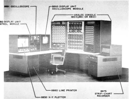
From Figures II-I, 11-2, and 11-3, it is obvious that analog computers differ
in physical appearance. The basic differences, however, lie much deeper.
Computers differ also in:
1) Capacity ••• the number of computing components
2) Capability ••• the quality of computing components and the
operations they perform
3) Reference Voltage Level .•• the operating voltage range of
the computer:
~ 10 or ~ 100 volts is typical
4) Convenience Factors .•• operator control, the accessibility of equipment, and others, some of which are less meaningful.
Since the basic principles of operation of all d-c general purpose analog computers are similar, the material presented in this chapter is applicable to any GPAC computing system.
Modern analog computers are equipped with removable patch panels which contain the input, output and control terminations of the various analog components in
a computer system. The input and output terminations of the components are
connected in a particular configuration which is defined by the problem being
solved. The control termination connections depend upon the mathematical
operation required of a particular component, and the manufacturers method of implementing the operating principles of that component. The term "patching" refers to the inter-connection of patch panel termination.
!:I~80 DISPLAY UNIT
CONTROL MODULE
8880 DISPLAY UNIT OSCILLOSCOPE MODULE
,...---ANALOG CONSOLE - - - " " ' \
{8810,8811 OR 88121
8860 LINE PRINTER 8875 STRIP-CHART
RECORDER
[image:28.613.30.474.213.555.2]Recommended programming symbols for the various components described in this
chapter are summarized on Pages 30-31 of this volume. These symbols may
re-quire slight modification to indicate specific component interconnections for a particular computing system.
C. Classification of Analog Components
Analog computer components, each of which performs a specific mathematical
operation, are classified either as linear or nonlinear components. The linear
components perform the mathematical operations of
1) multiplication by a constant
2) inversion
3) algebraic su~tion
4) continuous integration.;
These operations are sufficient to solve linear differential equations with constant coefficients.
The mathematical operations performed by nonlinear components are
1) multiplication and division of variables
2) the generation of arbitrary functions
3) the mechanization of constraints and elementary logic operations.
These components, together with the linear components, permit the analog computer to simulate the complex nonlinear systems which occur in practice.
1 • LINEAR COMPONENTS
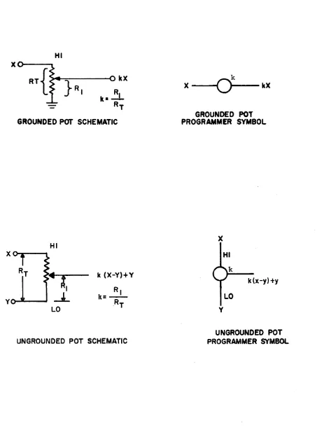
a. Attenuators---Multiplication of a d-c voltage by a 'positive constant
which is less than unity is accomplished by a potentiometer or pot,
also called an attenuator. This device, shown in Figure 11-4, is
simply a fixed resistor with a movable wiper arm. Carbon or wire
wound resistances which, for greater accuracy, have multiturn wiper arms are used in most computers.
Two types of pots, > "grounded" and "ungrounded
r;
a re used in modernanalog computers. These names are derived from the termination at
the bottom, or "LOri end, of the pot, as shown in the figure. The
total resistance of a pot is of the order of 2,000 to 30,000 ohms and depends on the design of the computer.
Grounded potentiometers are used in conjunction with a reference voltage (a constant voltage source equal to the upper limit of the computers operating voltage range) to obtain a fixed voltage less than reference voltage, or to multiply a problem variable by a
X
y
HI
GROUNDED POT SCHEMATIC
HI
k
(X-Y)+YRI
k =
-.RT LO
UNGROUNDED POT SCHEMATIC
X
---CO ...
k
_ -kX
GROUNDED POT PROGRAMMER SYMBOL
X
HI
k
k(x-y)+y
LO
Y
UNGROUNDED POT PROGRAMMER SYMBOL
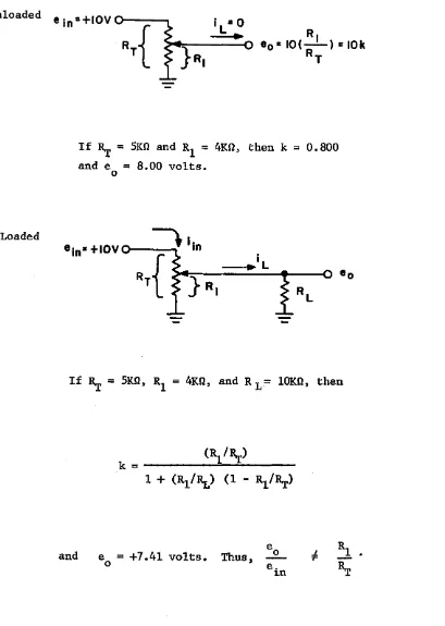
[image:30.613.64.524.72.686.2]Unloaded e In =+IOV I
a 0
....!:...
Loaded
If
Rwr
= 5Kn and Rl = 4Kn, then k = 0.800 and e = 8.00 volts.o
eln-
+IOVlJ----iL ---.~
If
Rwr
= 5Kn, Rl = 4Kn, and R L= lOKn, thenand
(l1.'R.r)
k = - - - = ...
-1
+
(Rl'~) (1 - Rl'Rr)eo e
=
+7.41 volts. Thus,o e.
~n
[image:31.615.72.481.122.697.2]at its top or "HIli end, and the resultant output is obtained through the wiper arm.
Figure 11-4 shows programmer symbols for both grounded and ungrounded pots.
The ungrounded pot has special applications in addition to the attenuation of two variables, indicated in Figure 11-4, which will be discussed in later chapters.
Normally, an analog computer will contain one and one-half as many pots as it has amplifiers, and 80% of these will usually be grounded.
i. Loading and Setting of Attenuators---the potentiometers shown in Figure 11-4 are "unloaded" which means that no current is being drawn through the wiper arm (i.e. they are feeding an infinite resistance-open circuit). Therefore, the mechanical ratio, B!/~, which can be set by a calibrated dial, is equal to its
electrical ratio, e
Ie. •
However, this is not the case wheno 1n
the infinite load is replaced by a finite load as shown in Figure 11-5.
In practice, the wiper arm of a pot will be 1I1ooking into" a load ranging from 103 to 106 ohms since a potentiometer generally feeds resistor inputs to operational amplifiers. The effect of a lOK* resistive load on a 5K pot set at 4/5 is shown in Figure 11-5.
In order to eliminate the effects of loading, potentiometers are set by monitoring the wiper voltage while the pot is "feeding" its normal load. In this way, it is possible to set potentio-meters to three or four places depending upon the precision of the monitoring device.
In most computers, each potentiometer has switching associated with it similar to that shown in Figure 11-6, below:
TO PRE - PATCH PANEL
HI TERMINATION
TO REFERENCE
VOLTAGE HI
Figure 11-6
*In these Notes, the follOWing notation is used:
3 6 3 6
to
WIPER PATCH PANELTERMINATION AND LOAD
*
When the switch is thrown, the patched input to the pot is replaced
by a reference voltage, and the loaded wiper arm is connected to a
monitoring device via a readout selector system. The readout device
can be either a high impedance, digital voltmeter (DVM) or a null meter.
The more sophisticated analog computer systems have digitally-set pots. Here, the potentiometer is selected through a pushbutton system, and then is set by a servo device also controlled by push buttons.
b. Operational Amplifiers---The operational amplifier is the basic unit
in the analog computer. It can be used in a "summing mode" to perform
any or all of the three linear operations: inversion, summation, and
nrultiplication by a constant. It also can be used in an "integrating
mode" to integrate a voltage or the sum of a number of voltages with respect to time.
Analog computer programs for investigating the behavior of physical systems require some operational amplifiers to be used as integraLors, while others are used as "sunnners," "inverters," "high gain
amplifiers," or in conjunction with special networks to perfonn nonlinear operations. Therefore, it is not necessary for all of the amplifiers to perform as integrators. In modern analog computers, a typical amplifier breakdown would be:
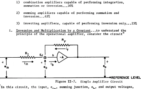
1) combination amplifiers capable of pe~forming integration,
su~tion or inversion ••• 30%
2) sunnning amplifiers capable of performing summation and
inversion ••• 45%
3) inverting amplifiers, capable of performing inversion only ••• 25%
i. Inversion and Multiplication by a Constant ••• to understand the principle of the operational amplifier, consider the circuit*
"4---if
b
+
Figure II-7. Simple Amplifier Circuit
In this circuit, the input, e. , surmning junction, eb , and output voltages,
e , are referred to a referen~R level, such as grouno. However, in the
igterest of simplicity, future circuits will omit the reference level terminal
and consider it to be grounded. The gain of the amplifier, -A, will also be
[image:33.613.33.506.376.677.2]where a high gain d-c amplifier (gain
=
-A) has a feedback resistor,~, and an input resistor, ~ (Figure II-7). The d-c amplifier is
designed so that
1) the amplifier output) e , is related to the summing junction voltage e
b, by the gainOof the amplifier (i.e., eo
=
-A ebwithin the reference voltage range of the computer),
2) the amplifier draws negligible current, ib
~10-9
amps, and3) the gain of the amplifier is extremely high, usually on the order of 108 at d-c.
Using Kirchhoff's laws, the nodal current equation at the s~ng junction,
SJ, is
or, from Ohm's law,
i :II:
b
Since ib ~, it can be neglected.
e.
+
eo = e~n 0
R:r
AR:r
Ali?
~
- - e e
=
R:r
in0
1
+
i
(~
+
1)
Replacing e b by
e
0
~
e
o
-A
we obtain:
Since the ratio of ~ to ~ usually is less than thirty, and A is much
greater than 1,
e
o =
~
-~ e. ~n (1)
From this equation we can see a most important character.istic of the operational amplifer: The input-output relationship is solely dependent on the ratio of the feedback to the input impedances (resistances).
Using this equation as a basis for discussion, some of the various uses of the operational amplifier can be illustrated.
When both resistors are of equal magnitude, R, the amplifier output voltage has the same amplitude as the input voltage but is of the opposite polarity. Thus, the mathematical operation of inversion is
e
o e. 1n
If the resistors are not of equal magnitude, the result is
multi-plication of the input by a constant. For example, if ~ were 1M
and
Rr
were lOOK,e o
~
= - - - eRI in
=
1M= _
10 - o.lM e inor. if the resistance ratio is inverted, e.
1n
eo
= -
""!O
e.
1n
ii. Summation---the addition of two parallel input resistors to the previous
circuit, yields
RF
'I .---~~---~
RI i l
•
4--ifR2 12
iln
•
-+eo
R3 i3
•
SJ 8b --+Ib
Figure II-B. Summing Amplifier Circuit
82 ---~~---~----~.---~
And, the SJ node equation,
i1
+
i2+
i3+
if - ib=
0 Using Ohm's law, this equation becomese
l - eb
+
e 2 - eb+
e 3 - eb+
e 0 - eb- ib
=
O.~
R2~
RfSince e
b and ib Qo< 0, we have
eo = -
[~
e1+
~
e2+
~
e3 ] • (2)If the number of input resistors is increased t~ say, N, the generalized
summer equation becomes
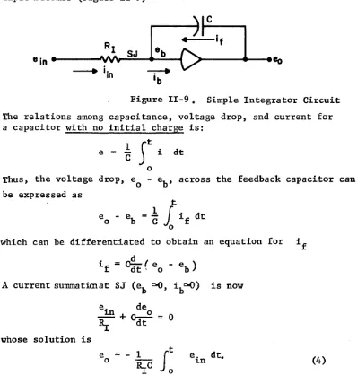
iii. Integration---when the feedback resistor used in previous circuits is replaced by a capacitor, the amplifier circuit for- a single input .becomes (Figure 11-9)
-gIC
1
RI
SJ
reb
~
ifein - ¥.I\;
-eo
---. iin --;-+
Ib
Figure 11-9. Simple Integrator Circuit
The relations among capacitance, voltage drop, and current for a capacitor with no initial charge is:
e
=
~
r
i dto
Thus, the voltage drop, eo - e
b, across the feedback capacitor can
be expressed as
t
eo - eb
=
~
1
if dto
which can be differentiated to obtain an equation for if
if =
o£t (
eo - e b )A current summatimat SJ (e
b ::.(), 'ib:::aoQ) is now
whose solution is
e. de
1n
+
~ = 011:
dte
o
= -
e. 1n dt. (4)We now have a device which can perform the operation of integration (with respect to time) on an input voltage.
For multiple resistor inputs, the integrator output is described by the equation:
+ --- +
~~]
dt (5) [image:36.612.121.519.112.530.2]iv. Generalized Amplifier Equations---if one defines the impedance, Z, of: a passive element as
Z
=
E Iwhere E is the voltage drop across the element, and I
current passing through it, the input-output expression for generalized circuit (Figure II-lO)is:
e o
ZF
Z I e. • ~n
SJ
is the the
Figure 11-10: Generalized Amplifier Circuit
For a multiple input amplifier circuit (Figure II-II),
SJ
J
Figure II-II: Generalized Multiple Input Amplifier Circuit.
*For simplicity further reference to ei(t), Z.(t), etc. will be considered
indi-the input-output relationship is
e o
n=N
n
=
1e
n
The impedance of a resistor is equal to its resistance in ohms
~ = R.
(6)
(7)
The impedance of a capacitor is time dependent. voltage drop across a capacitor is
Recalling that the
t
e
=
1
c
S
i dt o and defining the operatorst
P .5
d~
and 1 -J
p 0
dt, the
relation between voltage and current for a capacitor is
e =
..!..
pC
Since impedance is defined as the ratio of voltage drop to c~rrent,
the capacitor impedance is
= 1
~ (8)
v. Programming Symbo1s---before illustrating the programming symbols for the circuits just presented, it is important that one realizes how amplifiers and their associated passive elements are packaged
in modern day computers. Each amplifier hasl associated with it an
input network (resistors) and a feedback capacitor and/or resistor.
The input resistors are not equal in magnitude. Normally, one finds the input network containing from four to six resistors of two different magnitudes. For example, a six resistor input network may have three O.lM and three 1M resistors.
An inverter
R
e.
In >--...
--eo
whose overall gain is unity because it has identical input and feed-back resistors, is denoted by the programming symbol
e in - - I ...
C>>----
eg
If the passive elements were not identical the symbol would be
• Rf
where G is the resistance rat~o ~ •
In the case of summing amplifiers which can have multiple inputs, the programming symbol is
~
where G1 =
R '
I
~
=-R • 3
The symbol for an integrator, where G = l/~C ,
c
integrator becomes:
where G l =
..
-~
-2----'
e3-... ~
1 1 1
R C' G2 =~, and G3 = R C·
1 2 3
The V input to the top of
o
the integrator represents the initial value of e , or initial charge on
o
the feedback capacitor, which will be discussed in the next section of this chapter.
Finally, one may have occasion to use a high gain amplifier with an input network but without a feedback element
RI
'2 --.J\,fV'Ilr-~
This is commonly represented by the
>---'0
symbol
G1c>
'I G
2( >-_ _
82 - - -...
where Gl and G2 are inversely proportional to the size of the input
resistors.
To coordinate the packaging of amplifiers and passive elements with the symbols just presented, it must be realized that the input termi-nations of the input networks usually are not labeled with the
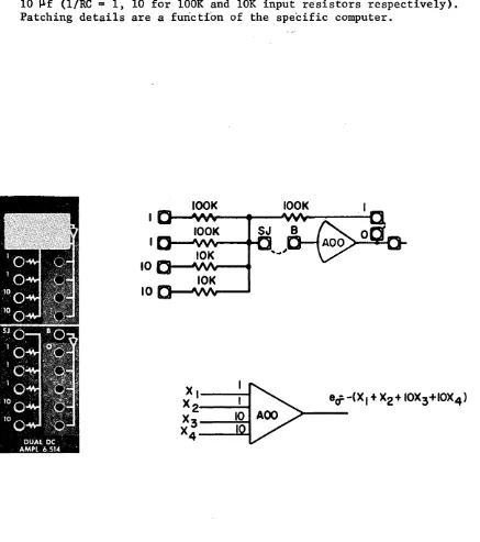
For example, consider the input or patch panel terminations for a PACE TR-48 computer shown in Figure 11-12. Each input labeled 10 is a 10K resistor. and each input labeled 1 is a lOOK resistor. Therefore, the standard feedback resistor for this system must be lOOK.
It follows, then, that if this notation is to be used throughout this computing system, the standard integrating capacitor must be 10 ~f (l/RC
=
1, 10 for lOOK and 10K input resistors respectively). Patching details are a furic tfon of the specific computer.10
10 10K
[image:41.613.82.519.206.699.2]vi. Drift
e" I
-
..
D-C amplifiers show a tendency to drift.* That is, the output does not necessarily remain steady and, in particular, does not necessarily
remain zero for zero input. This is due to changing characteristics
within the amplifier and, particularly, to changes in the first stage
of the amplifier. It is a most undesirable feature and can lead to
serious errors. To compensate for drift which might occur (i.e., to stabilize the d-c amplifier,) an a-c amplifier is used as shown in Figure 11-13.
I
Zf
l'
I
if
ZI
i· I ib D-C·0
-
'r.
-
AMPLIFIERIS
I
4",
A-CSTABILIZING -. .A.A ....
-
"'''':..1--L
AMPLIFIER'T
-Figure 11-13.
The effect of the a-c stabilizer is to increase the overall d-c' gain of the amplifier and further attenuate the drift of the operational amplifier by a factor equal to the gain of the a-c amplifier.
vii. Overload Indication -- If the amplifier is overloaded (required
out-put current or voltage is greater than design capabilities, eb
l
0, etc.)the overload signal connected to the output of the a-c amplifi.er is ex-cited. This overload indicator ensures that the computer is not used when errors exist due to operating the amplifiers beyond their capa-cities.
*
For a complete analysis of stabilization of the d-c amplifier,see "Introduction to Analogue Computers" by C.A.A. Wass, pages