Brushless doubly fed machine magnetic field distribution characteristics and their impact on the analysis and design

warwick.ac.uk/lib-publications

Manuscript version: Author’s Accepted Manuscript

The version presented in WRAP is the author’s accepted manuscript and may differ from the

published version or Version of Record.

Persistent WRAP URL:

http://wrap.warwick.ac.uk/127259

How to cite:

Please refer to published version for the most recent bibliographic citation information.

If a published version is known of, the repository item page linked to above, will contain

details on accessing it.

Copyright and reuse:

The Warwick Research Archive Portal (WRAP) makes this work by researchers of the

University of Warwick available open access under the following conditions.

Copyright © and all moral rights to the version of the paper presented here belong to the

individual author(s) and/or other copyright owners. To the extent reasonable and

practicable the material made available in WRAP has been checked for eligibility before

being made available.

Copies of full items can be used for personal research or study, educational, or not-for-profit

purposes without prior permission or charge. Provided that the authors, title and full

bibliographic details are credited, a hyperlink and/or URL is given for the original metadata

page and the content is not changed in any way.

Publisher’s statement:

Please refer to the repository item page, publisher’s statement section, for further

information.

1

Brushless Doubly Fed Machine Magnetic Field

Distribution Characteristics and their Impact on the

Analysis and Design

Mmamolatelo E. Mathekga, Sul Ademi and Richard A. McMahon

Abstract—This paper contributes to the characterisation of the brushless doubly fed induction machine (BDFIM), which is attractive as a variable speed generator in applications (off-shore wind turbine) with minimum maintenance requirements. The BDFIM has two three-phase stator windings of different pole numbers housed within the same stator slots and a short-circuited rotor winding capable of coupling fields of different pole numbers. The stator windings and rotor winding create a magnetic field distribution with a range of characteristics different to those of conventional induction machines. This paper presents an analysis to identify the field characteristics and discusses their impact on the analysis and design of the BDFIM. The characteristics are determined from an analysis of the sum of two rotating sinusoidal field waveforms and confirmed by comparison with time-stepping finite element results and measured magnetic flux density data.

Index Terms—Brushless doubly fed machine (BDFM), flux density, field distribution, rotor design, core loss, standing wave.

I. INTRODUCTION

B

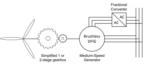
for use in wind turbines since they offer improved reli-ability and reduced capital and maintenance costs compared to the well-established doubly fed induction machine (DFIM) [1]. Employing BDFMs retains the low-cost advantage of the DFIM system as they only require a fractionally rated converter and they do not use permanent magnet materials [2], [3]. BDFMs have no brushed contact to the rotor, eliminating a maintenance requirement, making them particularly attractive for offshore wind turbines [4], [5]. In addition, they are intrinsically medium-speed machines, enabling the use of a simplified one or two stage gearbox. A schematic of a typical drivetrain is shown in Fig. 1.

There are two principle forms of BDFMs, namely the brushless doubly fed reluctance machine (BDFRM) [6], [7] and the brushless doubly fed induction machine (BDFIM) [4], which is the focal point of this paper. The brushless DFIM has its origins in the self-cascaded machine and has two non-coupling stator windings, referred to as the power winding (PW) and the control winding (CW) with different

pole numbers,p1 andp2, creating two fields in the machine

0

s magnetic circuit [8], [9]. A specially designed rotor couples to both stator windings.

The air-gap magnetic field distribution in the BDFIM has characteristics different to those of an electrical machine with a field distribution of a single pole number, the most obvious being that the form of the field distribution changes as a

Fig. 1. Brushless DFIM drivetrain set-up for wind power applications.

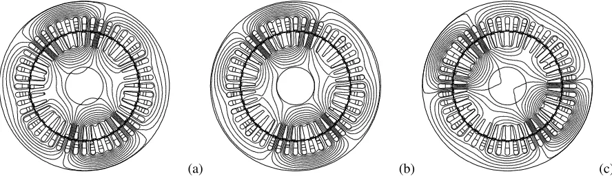
function of time as it rotates [10], as depicted in Fig. 2. From

a stator perspective, it does not have a clearly defined n

-pole pattern and that the movement of the field distribution is not a matter of simple rotation [11]. However, in early research work on the self-cascaded machine, the forerunner of the BDFIM, it was found that the field distribution had the interesting characteristic of being stationary in the rotor reference frame and that the amplitudes of the peaks in the field varied sinusoidally with angular position [12], [13].

As a consequence of the field distribution, conventional approaches cannot be used to predict core losses and determine saturation effects in the BDFIM. In particular it has been hard to establish a way of optimizing the magnetic design of these machines [10], [14]. Therefore, this paper examines the field distribution in a BDFIM to understand the impact of the nature of the field distribution on machine design and performance.

II. BDFIM MAGNETICFLUXDENSITYDISTRIBUTION

The radially directed air-gap flux density distribution is

found from the sum of the two principal fields with p1 and

p2 poles within the machine, assuming that space harmonics

components are small. In the stator reference frame the sum

of the two components, with p1 andp2 poles, is given by:

B(θ, t) =B1cos(2πf1t−p1θ)+B2cos(2πf2t−p2θ+α) (1)

whereB1andB2are the peak flux density of the2p1-pole and

2p2-pole components of the air-gap flux density, respectively,

f1 and f2 are the excitation frequencies, t is time, θ is the

angular position with a range of (0 : 2π)radians. The phase

offsetαis the combination of the relative physical position of

the two stator windings and the operating load angle. In summary, the form of the field distribution depends on the relative amplitude of the two field components, excitation frequencies and their relative angular offset. The field

[CC] Contours of A @ 0.8000000

[CC] Contours of A @ 0.8000000 [CC] Contours of A @ 0.8010000 [CC] Contours of A @ 0.8010000(a) [CC] Contours of A @ 0.8050000 [CC] Contours of A @ 0.8050000(b) (c) Fig. 2. The magnetic flux distribution of a BDFIM with a 4-pole and a 8-pole stator windings (Frame size D180), operating at 500 rpm in cascade mode with the 4-pole stator winding excited; captured 1 ms apart, in order.

non-sinusoidal function oft for allθvalues except in certain

special cases considered in section III-A, e.g., f1= 0 Hz or

f2= 0Hz. An example is shown in Fig. 3, illustrating changes

in flux density as function of θfor different values of t.

0 50 100 150 200 250 300 350

-2 -1.5 -1 -0.5 0 0.5 1 1.5 2

B (T)

 (Degrees)

t = 0.001 s

t = 0.002 s

t = 0.003 s

Fig. 3. Graphical representation of equation (1) as a function of θ for

consecutive values of t, 1 ms apart with: f1 = 50 Hz, f2 = 40 Hz,

B1= 1.0T, andB2= 0.7T.

III. FIELDANALYSIS

Equation (1) is a periodic function with a period, T, that is

given by

T = n

f1

= m

f2

(2)

where:nandmare integers that satisfy the following equation

n

m =

f1

f2

(3)

In certain circumstances the field distribution assumes par-ticular characteristics as considered below.

A. f1= 0Hz or f2= 0Hz

In this case equation (1) reduces to the sum of a traveling

waveform and a sinusoidal function of θ. The peak values of

B(θ, t) occur at varying angular positions at different times

because of the sinusoidal function ofθ, which contributes a θ

dependent offset to the peak value of the travelling waveform. However, the magnitudes of the peak values are independent of the angular position at which they occur.

B. Frequencies in the Ratio of the Poles

When the values off1 andf2 are related as follows

f1

p1

= f2 p2

(4)

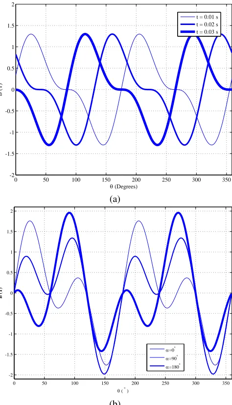
The form of the field distribution does not change as a

function of t and rotates around the machine as shown in

Fig. 4(a) because the angular velocities of the 2p1 and 2p2

pole flux density distributions are equal. However, the field

distribution as a function of θ, as well as the positive and

negative peak values, depend on the relative offsetαbetween

the2p1-pole and2p2-pole flux density distributions, which in

turn depends on operating conditions. Also, the positive and the absolute negative peak values are different and less than

|B1+B2| for most values of αas shown in Fig. 4(b).

C. Integer Ratio Frequencies

Under these conditions equation (1) reduces to the sum of

a traveling wave and a standing wave when the values of f1

andf2 are related byf1=±f2/iandf2=±f1/i, whereiis

an integer. For example when f1 =f2, equation (1) reduces

to

B(θ, t) = 2B1cos(2πf1t−0.5(p1+p2)θ)×cos(0.5(p2−p1)θ)

+ (B2−B1) cos(2πf1t−p2θ) (5)

The peak values of equation (5) are not equal at each angular position because of the standing wave term:

2B1cos (0.5(p2−p1)θ)×cos (2πf1t−0.5(p1+p2)θ)

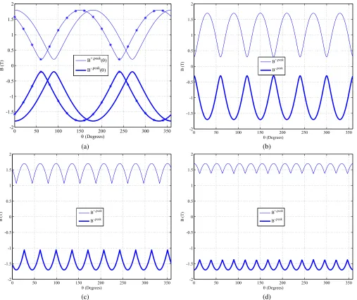
The peak values instead vary sinusoidally with angular position at any particular instant in time as shown in Fig. 5 and

Fig. 6; whereB−,peak_andB+,peak_{are the negative and positive}

peak values of equation (5) as a function ofθ. The amplitudes

at different θ values are not equal and vary periodically as

illustrated in Figs. 6(a) and 6(b) for two frequency ratios. The

general forms ofB−,peak_(θ)andB+,peak_{(θ)are deduced from}

Fig. 6 and they are given by:

B−,peak(θ) =−a0−a1|cos (kθ+β)| (6)

B+,peak_{(θ) = a}

3

0 50 100 150 200 250 300 350

-2 -1.5 -1 -0.5 0 0.5 1 1.5 2

B (T)

 (Degrees)

t = 0.01 s t = 0.02 s t = 0.03 s

(a)

0 50 100 150 200 250 300 350

-2 -1.5 -1 -0.5 0 0.5 1 1.5 2

 (  )

B (T)

=0

=90

=180

(b)

Fig. 4. Graphical representation of equation (1) as a function ofθwithf1

andf2values that are related by equation (4): (a) for consecutive values oft

10 ms apart, and (b) for different relative alignments withαequal to0,π/2,

andπradians.

where the values of a0,a1,k, and β vary with i as detailed

in section III(C) and as follows:

• k, the wavenumber, increases with increasing i. This

means that the number of angular positions where the

values of both B−,peak_{(θ) and B}+,peak_{(θ) are equal to}

−(B1+B2)and(B1+B2)respectively, is proportional

to the value of i.

• The value of a0 increases and that of a1 decreases

as i increases. This is despite their dependence on the

amplitudes of the 2p1 and2p2 flux density distributions

and it means that the variation of the positive and negative

peaks values of B(θ, t) with angular position becomes

less significant asi becomes large.

• β is equal to 90◦ and 0◦ for even and odd values of i,

respectively. This means that the angular positions where

the values of|B−,peak(θ)|and|B+,peak(θ)|are largest, are

not the same for even values of ias illustrated in Fig. 6

(a) and (b) as well as Fig. 6 (c) and (d).

0 50 100 150 200 250 300 350

-2 -1.5 -1 -0.5 0 0.5 1 1.5 2

 (Degrees)

B (T)

B+,peak

B-,peak

(a)

0 50 100 150 200 250 300 350

-2 -1.5 -1 -0.5 0 0.5 1 1.5 2

 (Degrees)

B (T)

B+,peak

B-,peak

(b)

Fig. 5. Graphical representation of the negative peak values (B−,peak_(θ))

and positive peak values (B+,peak_{(θ)) of equation (1) as a function ofθfor:}

(a)f2 = 0Hz,B1 = 1.0T, andB2= 0.5T as well as (b)f1 = 0Hz,

B1= 0.5T, andB2= 1.0T.

IV. CHARACTERISTICS WITHREFERENCE TO THEBDFIM

It is clear from section III that the field distribution depends

on the relationship between the frequencies of the2p1-pole and

2p2-pole stator excitations, i.e.f1andf2. In wind applications

the machine would be typically operated with one winding at grid frequency (50 or 60 Hz) with the other winding having a frequency range of around +/- 1/3 of grid frequency. However, in some applications both stator windings may be fed with variable frequencies.

A. Stator Reference Frame Field Distribution Characteristics and Implications

The values of f1 and f2 for the stator field distribution

components are related by the BDFIM speed equation:

N = 60f1±f2

p (7)

whereNis the shaft speed in rev./min. The only practical form

0 50 100 150 200 250 300 350 -2

-1.5 -1 -0.5 0 0.5 1 1.5 2

 (Degrees)

B (T)

B +,peak() B-,peak()

0 50 100 150 200 250 300 350

-2 -1.5 -1 -0.5 0 0.5 1 1.5 2

 (Degrees)

B

(T) B

+,peak

B-,peak

(a) (b)

0 50 100 150 200 250 300 350

-2 -1.5 -1 -0.5 0 0.5 1 1.5 2

 (Degrees)

B

(T) B

+,peak

B-,peak

0 50 100 150 200 250 300 350

-2 -1.5 -1 -0.5 0 0.5 1 1.5 2

 (Degrees)

B

(T) B

+,peak

B-,peak

(c) (d)

Fig. 6. Graphical representation of the negative peak values (B−,peak_{(θ)) and positive peak values (B}+,peak_{(θ)) of equation (1) as a function ofθfor: (a)} f2=f1, for alpha values equal to0andπ/6(*) radians (b)f2=−f1, (c)f2=f1/2and (d)f2=−f1/2.

opposite senses. The field distribution from a stator perspective will therefore exhibit all the characteristics presented in section III; i.e. the field distribution form changes as a function of time

(Fig. 2) except at speeds corresponding to values off1andf2

that satisfy equation (4).

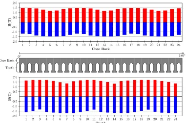
This latter characteristic is shown for the case satisfying section III-C by comparing the negative and positive peak flux density values computed across similar locations on different stator teeth and stator core back sections using a time-stepping finite element model of a prototype frame size D180 BDFIM

operating at a speed withf2=f1/2. The time-stepping finite

element simulation was performed following the approach in

[15] and the flux densities, B, in the teeth and core back

section were computed using the following equation:

B=Φ

A (8)

where A is the appropriate cross-sectional area and Φ is the

magnetic flux. Peak values are shown in Fig. 7 where it can be

seen that the peak flux density values vary periodically with angular position as in Fig. 6(b).

5

0◦ 180◦

Core Back

Tooth -2.0 -1.5 -1.0 -0.5 0.5 1.0 1.5 2.0

B(T)

1 2 3 4 5 6 7 8 9 10 11 12 13 14 15 16 17 18 19 20 21 22 23 24

Core Back

-2.0 -1.5 -1.0 -0.5 0.5 1.0 1.5 2.0

B(T)

1 2 3 4 5 6 7 8 9 10 11 12 13 14 15 16 17 18 19 20 21 22 23

Tooth

Figure 1: Rotor flux density levels. 1

Fig. 7. The computed negative and positive peak flux density values of different stator teeth and core back sections aligned to corresponding teeth and core

back sections for a finite element mode of frame size D180 BDFIM operating at 750 rev./min. withf1= 50Hz andf2= 25Hz at no load.

Fig. 8. System for measuring rotor flux density on the 250 kW BDFIM.

Fig. 9. System for measuring rotor flux density on the 250 kW BDFIM.

III-A and III-C as core loss will vary across different teeth and core back sections. Special consideration must go into the process of determining peak values from field distribution results obtained by simulation and by measurement as these peak values are position and load angle dependent.

B. Rotor Field Distribution Characteristics and Implications

The rotor current corresponding to the 2p1-pole and 2p2

-pole field components is single frequency when the BDFIM operates in the synchronous or cascade modes [20]. Also, the

relative space phase difference between the2p1-pole and2p2

-pole field components is fixed because they are generated by

the same winding. As noted on early work, the tooth flux densities depend on angular position as shown in Fig. 6(a) and Fig. 6(b); these are of course time varying at rotor current frequency. Maximum values occur at fixed angular locations. The above characteristics have been confirmed experimentally

TABLE I

DETAILS OF ANESTEDLOOPROTORFRAMESIZE OFD180 BDFMAND

250KW BDFIM.

Parameter Value

D180 BDFM 250 kW BDFIM

Frame size D180 D400

No. Rotor Slots 36 60

No. Stator Slots 48 72

No. Loops per. Nested Loop Set 3 5

by comparing the positive and negative peak flux density values in the rotor teeth and core back sections of two BDFIMs computed using finite element analysis with measured values. Both the frame size D180 and the 250 kW BDFIMs considered have 4-pole and 8-pole stator windings and a nested loop type of rotor whose details are given in Table I, using the approach in [16]. The flux density values were measured using a single turn flux coil wound around the tooth and core back sections. The voltage signal from the coil is integrated, sampled using a microcontroller and transmitted to a computer for processing

Core Back Tooth

0◦ 120◦

0.25 0.5 0.75 1.0

B/B

max

1 2 3 4 5 6 7 8 9 10 11 12 13 14 15 16 17 18 19

Tooth

0.25 0.5 0.75 1.0

B/B

max

1 2 3 4 5 6 7 8 9 10 11 12 13 14 15 16 17 18 19 20

Core Back

Figure 1: Rotor flux density levels.

1

(a) - 0 Nm

1 Image

This image

Core Back Tooth

0◦ 120◦

0.25 0.5 0.75 1.0

B/B

max

1 2 3 4 5 6 7 8 9 10 11 12 13 14 15 16 17 18 19

Tooth

0.25 0.5 0.75 1.0

B/B

max

1 2 3 4 5 6 7 8 9 10 11 12 13 14 15 16 17 18 19 20

Core Back

Figure 1: Rotor flux density levels.

1

(b) - 1000 Nm

Core Back Tooth

0◦ 180◦

0.5 1.0 1.5 2.0

B(T)

1 2 3 4 5 6 7 8 9 10 11 12 13 14 15 16 17

Tooth

0.5 1.0 1.5 2.0

B(T)

1 2 3 4 5 6 7 8 9 10 11 12 13 14 15 16 17 18

Core Back

Figure 1: Rotor flux density levels.

1

(c) - 0 Nm

Fig. 10. The computed negative and positive peak flux density values of different teeth and core back sections shown aligned to corresponding teeth and core

back sections, for: (a) and (b) - the 250 kW BDFIM operating at 625 rev./min. withf1= 50Hz andf2= 12.5Hz under different load conditions, and (c)

the frame size D180 BDFIM operating at 750 rev./min. withf1= 50Hz andf2= 25Hz at no load.

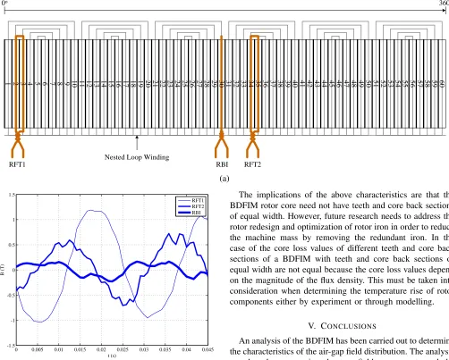
can be measured even when the rotor is rotating. A diagram of the rotor flux density measurement system is shown in Fig. 8, while the system installation and signal conditioning board was presented in Fig. 9 [21]. The computed and measured flux density values are shown in Fig. 10 and Fig. 11(b), respectively. The computed flux density peak values of the different teeth and core back sections are not all equal and their variation with angular position is consistent with that in Fig. 6(b). However, the computed flux density peak values in

7

6

5

4 7 8 9 10 11 12 13 14 15 16 17 20 21 22 23 24 25 26 27 28 29 31 32 33 38 39 40 41 42 43 44 45 46 47 48 49 50 51 52 53 54 55 56 57 58 59 60

RFT1

2

1 18 19

RFT2

37

36

35

34

3

0o ₃₆₀o

Nested Loop Winding

30

RBI

(a)

0 0.005 0.01 0.015 0.02 0.025 0.03 0.035 0.04 0.045 -1.5

-1 -0.5 0 0.5 1 1.5

B (T)

t (s)

RFT1 RFT2 RBI

(b)

Fig. 11. (a) - The location of search coils fitted on the 250 kW nested loop rotor BDFIM. RBI is the coil around the core back section of slot number 30, RTH1 and RTH2 are the flux coils around the rotor tooth numbers 3 and 35, respectively. The thick black lines represent the teeth. (b) - The measured flux density waveforms of two teeth and a core back section of the 250 kW BDFIM rotor at the locations shown in (a) with the excitation voltage of each stator winding set equal to 690 V and the machine operating at 680 rev./min. with a load torque of 3679 Nm.

are those measured across core back sections (Fig. 11(a)) between slots with conductor sections of the outer most loops of adjacent nested loop sets and teeth with the inner loop of each nested loop set.

Different operating conditions were used for the 250 kW BDFIM regarding the measured and computed flux density values. It is easy to appreciate that flux coil RBI in Fig. 11(b) measures the minimum flux density even though there is no other flux density measurement to compare with because the location on the core where the flux density was measured is consistent with the predicted location on the core back where the flux density is a minimum, and the peak flux density value measured with flux coil RFT1 was always greater than that measured with flux coil RFT2; also in agreement with predictions.

The implications of the above characteristics are that the BDFIM rotor core need not have teeth and core back sections of equal width. However, future research needs to address the rotor redesign and optimization of rotor iron in order to reduce the machine mass by removing the redundant iron. In the case of the core loss values of different teeth and core back sections of a BDFIM with teeth and core back sections of equal width are not equal because the core loss values depend on the magnitude of the flux density. This must be taken into consideration when determining the temperature rise of rotor components either by experiment or through modelling.

V. CONCLUSIONS

An analysis of the BDFIM has been carried out to determine the characteristics of the air-gap field distribution. The analysis was based on summing the two field components and the validity of the approach has been confirmed by experimental measurements in the machine and together with their impact the design of the machine. It has been found that:

1) The rotor and stator respective reference frames field distribution characteristics are generally different and that the stator field distribution characteristics depend on the combination of stator winding excitation frequencies and thus rotor speed as per equation (7).

2) The field distribution in the stator reference frame is always a non-sinusoidal function of angular position for different time instants, and it is also a non-sinusoidal function of time for different angular positions except when the stator winding excitation frequencies are equal or when either stator winding excitation frequency is equal to zero.

3) The field distribution form changes as a function of time always on the rotor and for most combinations of stator winding excitation frequencies except the combination that results in the two field distributions having the same angular velocity.

ACKNOWLEDGEMENTS

The authors would like to thank the Bradlow Foundation and St John’s College at the University of Cambridge for financial assistance.

REFERENCES

[1] R. McMahon, X. Wang, E. Abdi, P. Tavner, P. Roberts and M. Jagiela,

“The brushless DFIG as a generator in wind turbines,”Power Electronics

and Motion Control Conference, pp. 1859–1865, 2006.

[2] R. McMahon, P. Roberts, X. Wang and P. Tavner, “Performance of

BDFM as generator and motor,”IEE Proceedings Electric Power

Ap-plications, vol. 153, pp. 289–299, March. 2006.

[3] J. Carroll, A. McDonald and D. McMillan, “Reliability comparison of

wind turbines with DFIG and PMG drive trains,”IEEE Transactions on

Energy Conversion, vol. 30, pp. 663–670, March. 2015.

[4] H. Peng, M. Cheng, S. Ademi and M. Jovanovic, “Brushless

doubly-fed machines: Opportunities and challenges,”IEEE Chinese Journal of

Electrical Engineering, vol. 4, pp. 1–17, July. 2018.

[5] A. Oraee, E. Abdi, S. Abdi, R. McMahon and P. Tavner, “Effects of rotor

winding structure on the BDFM equivalent circuit parameters,”IEEE

Transactions on Energy Conversion, vol. 30, pp. 1660–1669, December. 2015.

[6] M. Hsieh, I. Lin and D. Dorrell, “An analytical method combining

equivalent circuit and magnetic circuit for BDFRG,”IEEE Transactions

on Magnetics, vol. 50, November. 2014.

[7] S. Ademi, M. Jovanovic and M. Hasan, “Control of brushless

doubly-fed reluctance generators for wind energy conversion systems,”IEEE

Transactions on Energy Conversion, vol. 30, pp. 596–604, 2015. [8] T. Strous, X. Wang, H. Polinder and J. Ferreira, “Brushless doubly

fed induction machines: Magnetic field analysis,” IEEE Transactions

on Magnetics, vol. 52, November. 2016.

[9] H. Gorginpour, H. Oraee and R. McMahon, “A novel modeling approach for design studies of brushless doubly fed induction generator based on

magnetic equivalent circuit,”IEEE Transactions on Energy Conversion,

vol. 28, pp. 902–912, 2013.

[10] X. Wang, P. Roberts and R. McMahon, “Optimisation of BDFM stator

design using an equivalent circuit model and a search method,”IET Int.

Conf. on Power Elect., Machines and Drives, pp. 606–610, 2006. [11] S. Williamson, A. Ferreira and A. Wallace, “Generalised theory of the

brushless doubly-fed machine. Part 1: Analysis,” IEE Proceedings

-Electric Power Applications, vol. 144, pp. 111–122, 1997.

[12] F. Creedy, “Some developments in multi-speed cascade induction mo-tors,”Journal of the Institute of Electrical Engineers, pp. 511–537, 1920.

[13] A. Arnold, “The two-speed cascade induction motor,” Journal of the

Institution of Electrical Engineers, vol. 63, pp. 1115–1122, 1925. [14] S. Abdi, E. Abdi and R. McMahon, “Optimization of the magnetic

circuit for brushless doubly fed machines,”IEEE Transactions on Energy

Conversion, vol. 30, pp. 1611–1620, 2015.

[15] M. Mathekga, S. Shiyi, T. Logan and R. McMahon, “Implementation of a PI phase angle controller for finite element analysis of the BDFM,”

Proc. of the Power Electronics, Machines and Drives, 2012.

[16] S. Abdi, D. Llano, E. Abdi and R. McMahon, “Experimental analysis

of noise and vibration for large brushless doubly fed machines,”The

Journal of Engineering, 2017.

[17] C. Steinmetz, “Operating alternating motors,”US587340, 1893.

[18] J. Pedro, A. Bastos and N. Sadowski, “Electromagnetic modelling by

finite element methods,”Marcel Dekker Inc., New York, 2003.

[19] A. Bousbaine, “An investigation into the thermal modelling of induction

motors,”Department of Electronic and Electrical Engineering,

Univer-sity of Sheffield, 1993.

[20] A. Wallace, R. Spee and G. Alexander, “The brushless doubly-fed

machine: Its advantages, applications and design methods,”IEEE. 6th

Int. Conf. Electrical Machines and Drives, pp. 511–517, 1993. [21] D. Llano, S. Abdi, M. Tatlow, E. Abdi and R. McMahon, “Energy

har-vesting and wireless data transmission system for rotor instrumentation

in electrical machines,”IET Power Electronics, vol. 10, pp. 1259–1267,