Impulse response modeling for underwater optical wireless channels

warwick.ac.uk/lib-publications

Original citation:

Li, Yiming, Leeson, Mark S. and Li, Xiaofeng (2018) Impulse response modeling for

underwater optical wireless channels. Applied Optics, 57 (17). pp. 4815-4823.

doi:

10.1364/AO.57.004815

Permanent WRAP URL:

http://wrap.warwick.ac.uk/103031

Copyright and reuse:

The Warwick Research Archive Portal (WRAP) makes this work by researchers of the

University of Warwick available open access under the following conditions. Copyright ©

and all moral rights to the version of the paper presented here belong to the individual

author(s) and/or other copyright owners. To the extent reasonable and practicable the

material made available in WRAP has been checked for eligibility before being made

available.

Copies of full items can be used for personal research or study, educational, or not-for-profit

purposes without prior permission or charge. Provided that the authors, title and full

bibliographic details are credited, a hyperlink and/or URL is given for the original metadata

page and the content is not changed in any way.

Publisher’s statement:

© 2018 Optical Society of America. Users may use, reuse, and build upon the article, or use

the article for text or data mining, so long as such uses are for non-commercial purposes and

appropriate attribution is maintained. All other rights are reserved.

A note on versions:

The version presented here may differ from the published version or, version of record, if

you wish to cite this item you are advised to consult the publisher’s version. Please see the

‘permanent WRAP URL’ above for details on accessing the published version and note that

access may require a subscription.

Research Article

Impulse Response Modeling for Underwater Optical

Wireless Channels

Y

L

, M

S. L

,

X

L

1_{School of Astronautics and Aeronautics, University of Electronic Science and Technology of China, Chengdu, Sichuan, 611731 China} 2_{School of Engineering, University of Warwick, Coventry, CV4 7AL UK}

*_{Corresponding author: [email protected]}

In underwater optical wireless communication (UOWC) channels, impulse response is widely used to de-scribe the temporal dispersion of the received signals. In this paper, we propose a new function to model the impulse response in most realistic cases in the UOWC channels. By exploiting the inherent properties of such channels, our newly proposed model is superior to the conventional weighted double Gamma functions (WDGF) model in explaining the behavior of the channel. We use Monte-Carlo simulation to verify that our newly proposed model has a better accuracy of numerical fitting in most cases. Therefore, this new modeling approach offers a more convenient way to evaluate the performance of different kinds of UOWC channels. © 2018 Optical Society of America

OCIS codes: (010.4455) Oceanic propagation, (010.4458) Oceanic scattering, (290.4210) Multiple scattering.

http://dx.doi.org/10.1364/ao.XX.XXXXXX

1. INTRODUCTION

Underwater optical wireless communication (UOWC) systems have received a great deal of attention due to the advantages of a much higher data rate, security, and a much lower latency compared to the traditional underwater acoustic communica-tion systems. Although the transmit length is relatively short as the light beam suffers from absorption, scattering and tur-bulence induced fading, UOWC is still a promising technology in many applications such as the underwater wireless sensor networks (UWSNs) to satisfy the increasing demands for ocean exploration with high data rate transmission [1].

Prior studies have shown that the optical beam will suffer from absorption and scattering, the properties of which can be described by the inherent optical properties (IOPs) of the water [2]. The absorption will cause an inevitable power loss and therefore the blue-green spectrum is used due to its minimum absorption by seawater. On the other hand, the scattering effect will change the direction of the transmit beams. In a turbid environment such as coastal and harbor waters, the photons will be undergo scattering more than once. This effect is called the multiple scattering effect which is studied in [3] and exerts a positive impact on the overall received power [4]. However, this effect will also increase the temporal dispersion which is a negative impact, particularly in very turbid water (e.g. harbor and coastal water).

On the other hand, the optical beam will also suffer from tur-bulence induced fading, which is caused by the random changes of water temperature and salinity, as well as the randomly

dis-tributed air bubbles in the water [5–10]. Moreover, experiments have shown that turbulence can be separated from particle scat-tering and absorption [11]. Therefore, it is reasonable to treat these two effects separately to reduce the complexity of the anal-ysis.

In this paper, we focus on the temporal dispersion of the fading-free line-of-sight (LOS) UOWC channel and investigate the channel impulse response in turbid water. Recently, Monte-Carlo simulations have been carried out to analyze the properties of the impulse response in UOWC channels [12–15]. Further-more, there has also been comparison of the Monte-Carlo results with Mullen’s experimental study to validate the efficiency of the simulation results [13,16]. Inspired by Mooradian’s work on modeling the impulse response in clouds by the double Gamma functions (DGF), Tang applied the DGF to model the impulse response in UOWC links [17]. Moreover, Dong and Zhang mod-ified the DGF model by adding parameters and terms to apply it to multiple-input-multiple-output (MIMO) UOWC channels [18,19].

Research Article

curve fitting process. To the best of our knowledge, no previous work has attempted to explain the connections between the IOPs and the impulse response models. In this work, we focus on explaining such questions and proposing a new model to fit the impulse response in most realistic situations. We also conclude by numerical results that the newly proposed model is superior to Dong’s model in most cases. Moreover, we can also explain the similarities and differences of the impulse response in differ-ent types of water by the natural decomposition of absorption and scattering in our model. This provides a better approach to the estimation and analysis of the characteristics of UOWC channels.

This paper is organized as follows: Section2describes the optical characterizations and the scattering phase functions of seawater. In Section3we describe the basic rules of our Monte-Carlo simulation as well as discussing our newly proposed model. Simulation results and data analysis are presented in Section4followed by conclusions in Section5.

2. PRELIMINARIES

A. Optical Characterizations of Seawater

According to Mobley’s statement [2], absorption and scattering are two major effects in the underwater optical channel. The for-mer will cause an inevitable loss of optical power by converting it into other forms such as heat. Meanwhile, the latter arises from the interaction of photons with the small particles in the water and will change the transmission path of the light. The energy loss caused by these two effects can be expressed by the absorp-tion coefficienta(λ)and the scattering coefficientb(λ)

respec-tively. Moreover, the attenuation coefficientc(λ) =a(λ) +b(λ)

is also defined to describe the overall energy loss in the channel. It is worth mentioning that the values ofa(λ),b(λ)andc(λ)

will vary with the water type as well as the wavelength of the lightλ.

B. Scattering Phase Function of Seawater

Unlike the optical wireless communication channel in the at-mosphere, the light in the underwater optical channel will en-counter a large number of particles and the scattering effect will be much more significant. As a consequence, multiple scatter-ing effects will play a significant role in the received power. To study this kind of phenomenon, the scattering phase function (SPF) β(λ,θ,φ)is introduced to describe the energy

distribu-tion of the scattering effect, whereθis the polar angle andφis

the azimuthal angle of the scattering respectively. The SPF is constrained so that:

Z2π

0

Z π

0 β(λ,θ,φ)sin(θ)dθdφ=1. (1)

Moreover, it is often assumed that the particles are spherical and the scattering is azimuthally symmetric. Therefore, Eq. (1) can be rewritten as:

2π Z π

0 β

(λ,θ)sin(θ)dθ=1, (2)

where the 2πcomes from the integral over the azimuthal angle.

Several models have been proposed to describe the SPF of the underwater environment. Among them there are two most widely used models.

The first is the long-standing Henyey-Greenstein phase func-tion (HGPF) which was first proposed by Henyey to describe

the scattering effect in astrophysics [20]. This can be expressed as:

βHG(θ) = 1−g

2

4π(1+g2−2gcos(θ)) 3 2

, (3)

wheregis the average cosine ofθ. Although this is very

conve-nient for numerical calculation and acceptable to approximate the shape of the actual phase function in a multiple scattering channel, it differs from Petzold’s long established measurements [21] in both small forward angles (θ<20◦) and large backward

angles (θ > 130◦) [22]. Therefore, use has been made of the

Two-Term HGPF to improve the fitting performance. Although this does indeed enhance the fit, it also underestimates Petzold’s measurement whenθ<1◦because of the inherent property of

such functions in small angle situations.

As a result, the HGPF has now been supplanted by the more complicated but more realistic and widley used Fournier-Forand phase function (FFPF). This was derived by Fournier and Forand as an approximate analytic form under two assumptions [23]. Firstly, the particles have a hyperbolic size distribution. Sec-ondly, each particle scatters according to the anomalous diffrac-tion approximadiffrac-tion to the exact Mie theory. By applying the two approximations to the analytic form, the FFPF can also reveal some of the inherent properties of the underwater channel. The phase function is given by [24]:

βFF(θ) = 1

4π(1−δ)2δν

{ν(1−δ)−(1−δν)

+ [δ(1−δν)−ν(1−δ)]sin−2

θ

2

+ 1−δ

ν 180 16π(δ180−1)δν₁₈₀

3cos2(θ)−1

,

(4)

whereν = 3−₂µ andδ = 4

3(n−1)2sin

2θ

2

. Hereνis the slope

parameter of the hyperbolic distribution,nis the refractive index of the water, andδ180isδevaluated atθ=180◦.

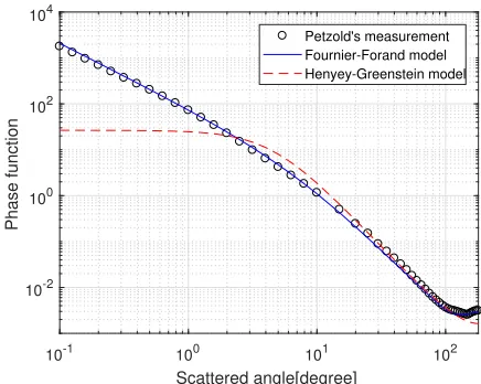
We illustrate the performance of the two models by compari-son with the experimental data from Petzold’s previous work [21]. Thus, the comparison of the HGPF, the FFPF and Petzold’s experimental data is shown in Fig.1. As may be seen in Fig.1,

10-1 100 101 102

Scattered angle[degree]

10-2 100 102 104

Phase function

Petzold's measurement Fournier-Forand model Henyey-Greenstein model

Fig. 1.Comparison of different phase functions.

phase functions in the underwater environment than the HGPF, especially at very small angles. Therefore, we apply the FFPF to model the scattering effect in the rest of this paper.

3. IMPULSE RESPONSE MODELING

A. Monte-Carlo Simulation

To fully explore light propagation in the underwater environ-ment it is necessary to solve the radiative transfer equation (RTE) [2]. Analytical solutions of the RTE are only available for a limited range of geometries and so Monte-Carlo Simulation is widely used to evaluate underwater channel performance. The method is much more convenient for application to the under-water environment given the paucity of analytical results for the RTE.

We adopt a Monte-Carlo approach similar to Cox and Tang’s previous work [12,17]. However, their modeling utilized the synthesis law of Poisson processes but violated the decomposi-tion law of Poisson processes. Therefore, our Monte-Carlo simu-lation is modified in the transmission part to make it consistent with the definition of the absorption and scattering coefficients in [25]. On the other hand, we have also introduced some mod-ifications in the receiving part to obtain a stabler result when analyzing the off-axis situation. The illustration of our system is shown in Fig.2.

X

Y

Z z

x

y

x y

z

x z

y

t0

Fig. 2.The illustration of the Monte-Carlo Simulation.

The Monte-Carlo simulation of the system, which is illus-trated in Fig.2, is composed of three main parts: the initial part, the transmission part, and the receiving part.

In the initial part, we consider the collimated laser-based source. And the photon position is set at the origin of the Carte-sian coordinates(x0,y0,z0) = (0, 0, 0)and the photon emission angle is set as(θ0,ϕ0) = (0, 0).

In the transmission part, the light will travel for a random distance obeying a negative exponential distribution, which can be expressed as:

p(∆s) =b·e−b∆s. (5)

Therefore, the distance of the transmission path can be gener-ated by:

∆s=−ln(1−U[0, 1])

b , (6)

whereU[0, 1]is a uniformly distributed random variable.

Then the light will encounter a scattering effect. The zenith angle can be generated as follows. Firstly, the piecewise nu-merical approximation of the cumulative distribution function (CDF)FFF(θ)can be calculated by using Eq. (4). Secondly, a

uniform distributed random numberX∼U[0, 1]can be gener-ated. Thirdly, we can generate the zenith angle by applying the equation:

θ=F_FF−1(X). (7)

And the azimuth angle can be obtained by:

ϕ=2π·U[0, 1]. (8)

Meanwhile, the light will also suffer from the attenuation ef-fect, and the power remaining before thenth_{scattering can be}

expressed as:

Pn=Pn−1·e−a∆s. (9) We should also transfer the zenith angle and the azimuthal angle into Cartesian coordinates. In this step, we allow as many as 300 scattering events to ensure that more than 99 percent of the paths are received in our simulation. Moreover, we have verified that this value is sufficient for all scenarios in this paper.

According to the analysis above, the absorption and the scat-tering effects have independent influences on the transmitted light. By distinguishing the differences between these two ef-fects, we can analyze them separately in different steps. The first step is to construct the scattering path of the photon without con-sidering the absorption effect. The second step is to calculate the absorption effect directly using the path length generated by the first step and Eq. (9). This will also influence our understanding of the impulse response modeling in Sec.3.B.

It is worth mentioning that the scattering path is determined by the scattering effect rather than the absorption effect. In-spired by this phenomenon, we introduce the term “scattering length" which is defined asbLin this paper. This is utilized to substitute the commonly used term “attenuation length" which is defined ascL, whereLis the transmission distance between the transmitter and the receiver. In what follows, it is much more convenient to compare different water types by the application of this scattering length.

In the receiving part, we generalize the simulation and adapt it to both the on-axis and the off-axis situations. In order to achieve this goal, we have improved the structure of the simu-lation system which is shown in Fig.2. Assuming the circular symmetric property of the azimuthal angle, we can collect all the photons reaching the receiving spherical surface with a radius ofLand an off-axis zenith angle ofθt ∈[θt0−∆θt0,θt0+∆θt0] to estimate the performance of the receiver which is located at a distance ofLand an off-axis zenith angle ofθt0with a radius ofr0=∆θt0L(whenθt0 ≤∆θt0, the closed interval will be re-duced to[0, 2∆θt0]and thus represent the on-axis situation). By applying this system, we can collect more photon paths when analyzing the off-axis situation so as to help us to obtain a sta-bler simulation result. It is worth mentioning that we should also normalize the receiver aperture when comparing the data. Moreover, only the photons within the receiving area as well as arriving from angles less than half of the receiver field-of-view (FOV) can be detected.

B. Functions for Impulse Response Modeling

Double Gamma functions (DGFs) have first been adopted to model the impulse response in clouds by Mooradian [26]. The form of such a function can be written as:

whereC1,C2,C3, andC4are the four parameters to be solved;

∆t =t−t0 >0, wheretis the time scale andt0 = L/vis the non-scattering propagation time which is the ratio of the link rangeLover the light speed in waterv.

Inspired by the dispersive nature of both cloud and underwa-ter channels, Tang applied double Gamma functions to model the impulse response in UOWC links [17]. However, such func-tions are only applicable with relatively large values of the atten-uation length where the multiply scattered light is dominant. In order to generalize these functions, Dong added 2 parameters to the double Gamma functions and proposed the weighted double Gamma functions (WDGF) [18]:

h(t) =C1∆tαe−C2∆t+C3∆tβe−C4∆t, (11) whereαandβare the 2 newly added parameters to be

deter-mined. Eq. (11) is applicable for both small and large values of the attenuation length. Moreover, it is also applicable to model a 2×2 UOWC MIMO channel with a relatively large attenua-tion length. This funcattenua-tion has also been extended to the general MIMO UOWC channel by Zhang [19].

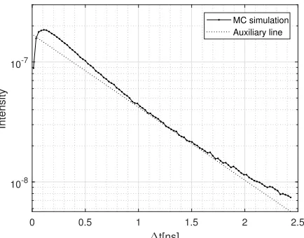
However, by carefully inspecting the results of the Monte-Carlo simulation which is plotted on a logarithmic scale as Fig.3, we can conclude that the tail of the impulse response should

0 0.5 1 1.5 2 2.5

t[ns]

10-8

10-7

Intensity

MC simulation Auxiliary line

Fig. 3.Monte-Carlo simulation of impulse response in harbor water. L=10.93 m, FOV=40◦.

be convex. This phenomenon implies that the tail decays more slowly than the exponential function. However, the weighted Gamma function is a strictly concave function. Although a fit can be made to the experimental data using Eq. (11), it will constantly underestimate the intensity of the tail because of this difference of convexity.

Inspired by the above mentioned problem, we propose a new function which can be written in the form of a combination of exponential and arbitrary power function (CEAPF) as below:

h(t) =C1 ∆ tα

(∆t+C2)β

·e−a·v(∆t+t0)_{, (12)}

whereC1>0,C2>0,α>−1, andβ>0 are the four

param-eters to be found andvis speed of light in water. To ensure that the function tends to 0 when∆tapproaches infinity with arbitrary attenuation coefficientawe need to also apply the constraintβ > α. These parameters can be calculated from

Monte-carlo simulation results using the nonlinear least square criterion as:

(C1,C2,α,β) =arg min

Z

[h(t)−hmc(t)]2dt

, (13)

whereh(t)is the CEAPF model in Eq. (12) andhmc(t)is the

results of the Monte-Carlo simulations.

It is easy to compare the CEAPF to the WDGF. Some of the most important conclusions are listed as below:

B.1. Convexity

We can rewrite Eq. (12) as:

ln[h(t)] =lnC1+αln∆t−βln(∆t+C2)−a·v(∆t+t0). (14)

The second derivative of Eq. (14) is:

d2_ln[h(t)] d∆t2 =−

α ∆t2+

β

(∆t+C2)2. (15)

When∆tis sufficiently large, which is the situation of the tail, CEAPF will be convex in accordance with the simulation result.

B.2. Decomposition of Absorption and Scattering

Since absorption and scattering are two independent effects in the underwater optical channel, the form of our newly proposed model naturally decomposes these two effects.

Absorption will convert optical power into other forms; this effect can be expressed by Eq. (9). By multiplying all the power loss of a certain trace, we can interpret the exponential term of Eq. (12) as the total loss of the trace.

On the other hand, the scattering effect will influence the distribution of the length of the received traces, and we can de-scribe it by the arbitrary power term of Eq. (12). Specifically,C1 describes the amplitude of the impulse response, the numera-tor of the term describes the rising edge and the denominanumera-tor contributes to the falling edge of the function.

Moreover, by rewriting Eq. (12) as

h(t) =C₁0 (b∆L) α

(b∆L+C0

2)β

·e−ab·b∆L·_e−ab·bL_{, (16)}

where∆L = v∆t, C₁0 = (bv)β−α_C

B.3. Accuracy of the Estimation

By exploiting the inherent properties of the simulation results, we can expect a more accurate estimation than the WDGF model when applying our CEAPF model. As a result, when the mul-tiple scattering effect dominates, and the transmit and receive apertures are precisely aligned, the performance of our newly proposed model is better in the sense of root-mean-square devia-tion (RMSE). Moreover, the CEAPF model will do a much better job when we are trying to predict the power in the tail.

Nevertheless, the CEAPF is also applicable for fitting the impulse response of a relatively smaller scattering length where the trajectory path still plays a significant role. Moreover, the CEAPF is able to accurately capture the off-axis behavior.

All the above mentioned scenarios are discussed in detail in Sec.4.

B.4. Efficiency of the Estimation

Compared to the WDGF model with 6 parameters, the CEAPF model with 4 parameters can be computed more quickly when using the nonlinear least square criterion.

B.5. Integrability

In order to calculate the overall received power, we may need to integrate the CEAPF. By using Eq. (3.383.5.11) in [27], and then representing the Laguerre polynomials by confluent hypergeo-metric functions, which are standard built-in functions in most well-known mathematical software packages, given by:

1F1(a;b;z) =

∞

∑

a(n)_zn

b(n)_n!, (17)

wherea(0)=1 anda(n)=a(a+1) (a+2)· · ·(a+n−1)when n6=0, we can represent the overall received power as:

P=C1e−aL·π·csc((α−β)π) ·

(

C1₂+α−βΓ(1+α)1F1(1+α; 2+α−β;avC2)

Γ(β)Γ(2+α−β)

−(av) −1−α+β

1F1(β;−α+β;avC2)

Γ(−α+β)

)

,

(18)

where Re{a}>0, Re{α}>−1, and Re{C2}>0. And all these constraints are consistent with our assumptions.

4. NUMERICAL RESULTS

We consider a UOWC system with 514 nm wavelength to cor-respond with that used in [21] and a photon detector with an aperture of 40 cm in diameter. Moreover, we choose a collimated source to receive the maximum power as would customarily be the case in experimental systems. On the other hand, we choose a typical value ofv = 2.237×108 _{m/s as the speed of light} in water. The Monte-Carlo simulation is depicted in Sec.3.A; 109transmissions are simulated to obtain the impulse response hMC(t)using MATLAB. Based on the settings above, we

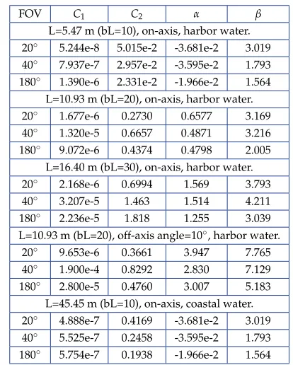
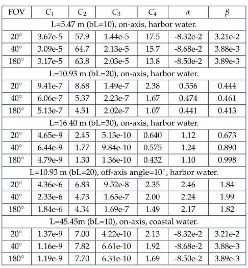
sim-ulated the beam propagation for a range of link lengths, FOVs and off-axis angles in coastal (a=0.179m−1,b =0.220m−1) and harbor (a = 0.366m−1_{,b = 1.829m}−1_{) water. We then} produced a fit to the impulse response using Eq. (12) with the nonlinear least square criterion depicted by Eq. (13). The pa-rameters of the CEAPF and WDGF are listed in TABLE1and TABLE2respectively.

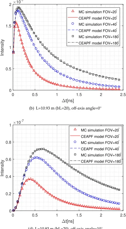
Fig.4shows the normalized impulse response for FOV val-ues of 20◦, 40◦and 180◦in harbor water. Fig.4demonstrates

Table 1.parameters of CEAPF in different UOWC channels

FOV C1 C2 α β

L=5.47 m (bL=10), on-axis, harbor water.

20◦ 5.244e-8 5.015e-2 -3.681e-2 3.019

40◦ 7.937e-7 2.957e-2 -3.595e-2 1.793

180◦ 1.390e-6 2.331e-2 -1.966e-2 1.564

L=10.93 m (bL=20), on-axis, harbor water.

20◦ 1.677e-6 0.2730 0.6577 3.169

40◦ _{1.320e-5 0.6657 0.4871 3.216}

180◦ _{9.072e-6 0.4374 0.4798 2.005}

L=16.40 m (bL=30), on-axis, harbor water.

20◦ 2.168e-6 0.6994 1.569 3.793

40◦ 3.207e-5 1.463 1.514 4.211

180◦ 2.236e-5 1.818 1.255 3.039

L=10.93 m (bL=20), off-axis angle=10◦, harbor water.

20◦ 9.653e-6 0.3661 3.947 7.765

40◦ 1.900e-4 0.8292 2.830 7.129

180◦ 2.800e-5 0.4760 3.007 5.183

L=45.45 m (bL=10), on-axis, coastal water.

20◦ 4.888e-7 0.4169 -3.681e-2 3.019

40◦ _{5.525e-7 0.2458 -3.595e-2 1.793}

180◦ _{5.754e-7 0.1938 -1.966e-2 1.564}

that the CEAPF fits well with the simulated impulse response regardless of the propagation distance, FOV and off-axis angle. We set thebLproduct to be 10, 20 and 30, and these represented propagation distances of 5.47 m, 10.93 m and 16.40 m with on-axis impulse response results as shown in Fig.4(a), (b) and (c) respectively. We can firstly conclude from these figures that the impulse response is more dispersive asLincreases, which would be expected intuitively because the photons suffer more scatter-ing over a longer propagation distance. Secondly, the impact of the FOVs will also increase with a largerLfor the same reason. Thirdly, the received power will decrease with an increasing propagation distance as the photons undergo more attenuation. On the other hand, the impulse response of an off-axis angle of 10◦is shown in Fig.4(d). By comparing Fig.4(b) and (d), we can also conclude that the impulse response disperses more heavily on an off-axis angle than an on-axis angle. Simultaneously, the received power will decrease on an off-axis angle due to the misalignment.

Moreover, in a typical situation of turbid water with a rel-atively long transmission distance of 10.93 m and a relrel-atively small receiver FOV of 20◦, a comparison between our result and the WDGF fitting result given by Eq. (11) is shown in Fig.5. We can conclude from Fig.5that in such a situation, the CEAPF model performs better than the WDGF model, especially in the “tail” area. This result is in accordance with our analysis in Sec.3.B. Although this phenomenon is not always pronounced enough to be shown in figures, we can numerically compare our results with the WDGF fitting results. On one hand, We apply the rooted-mean-square deviation (RMSE) criterion, which is also used in Tang’s previous work [17], to compare the overall performance. The RMSE criterion can be written as:

RMSE=

v u u t

N

∑

0 0.02 0.04 0.06 0.08 0.1

t[ns]

0 1 2 3 4 5 6 7 8

Intensity

10-5

MC simulation FOV=20°

CEAPF model FOV=20° MC simulation FOV=40° CEAPF model FOV=40°

MC simulation FOV=180° CEAPF model FOV=180°

(a) L=5.47 m (bL=10), off-axis angle=0◦

0 0.5 1 1.5 2 2.5

t[ns] 0

0.5 1 1.5 2

Intensity

10-7

MC simulation FOV=20°

CEAPF model FOV=20° MC simulation FOV=40° CEAPF model FOV=40°

MC simulation FOV=180° CEAPF model FOV=180°

(b) L=10.93 m (bL=20), off-axis angle=0◦

0 1 2 3 4 5 6 7

t[ns] 0

0.5 1 1.5 2 2.5

Intensity

10-9

MC simulation FOV=20° CEAPF model FOV=20°

MC simulation FOV=40° CEAPF model FOV=40°

MC simulation FOV=180°

CEAPF model FOV=180°

(c) L=16.40 m (bL=30), off-axis angle=0◦

0 0.5 1 1.5 2 2.5

t[ns]

0 0.2 0.4 0.6 0.8 1

Intensity

10-7

MC simulation FOV=20°

CEAPF model FOV=20°

MC simulation FOV=40°

CEAPF model FOV=40°

MC simulation FOV=180°

CEAPF model FOV=180°

(d) L=10.93 m (bL=20), off-axis angle=10◦

Fig. 4.Impulse response in harbor water.

where∆t0 is the unit time interval, N is the number of time intervals,hmc(·)represents the impulse response obtained by

Monte-Carlo simulation, andh(·)represents Eq. (11) when ap-plying the WDGF and Eq. (12) when apap-plying the CEAPF. On the other hand, in order to emphasize the improvement in esti-mating the tail of the impulse response, we also compared the power deviation of the tail (PDT), which can be written as:

PDT= Ptail,h−Ptail,MC

Ptail,MC

×100%, (20)

wherePtailrepresents the overall power of the tail which is

be-yond the scope of the figures,Ptail,his calculated from the fitting

curve, andPtail,his calculated from the Monte-Carlo simulation

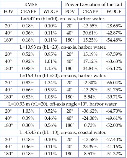
result. The numerical results corresponding to Fig.4are listed in TABLE3. We can conclude from TABLE3that the CEAPF model is better in most listed cases in the sense of RMSE. But the numerical data of Fig.4(a) shows that the performance of the CEAPF model is slightly worse than the WDGF model in the sense of RMSE, but both error values are very small (≤0.36%), effectively negligible. On the other hand, the numerical data of Fig.4(d) shows that the performance of the CEAPF model

is slightly worse only in the case of FOV = 20◦. As a result, the maximum RMSE deviations of the CEAPF model and the WDGF model are 1.03% and 1.34% respectively in all the cases listed in this paper. Moreover, the RMSE deviation of the DGF model is reported to be less than 5% in Tang’s previous work (the maximum deviation listed is 4.276%, which is much larger than the CEAPF model) [17].

Table 2.parameters of WDGF in different UOWC channels

FOV C1 C2 C3 C4 α β

L=5.47 m (bL=10), on-axis, harbor water.

20◦ 3.67e-5 57.9 1.44e-5 17.5 -8.32e-2 3.21e-2

40◦ 3.09e-5 64.7 2.13e-5 15.7 -8.68e-2 3.88e-3

180◦ 3.17e-5 63.8 2.03e-5 13.8 -8.50e-2 3.89e-3

L=10.93 m (bL=20), on-axis, harbor water.

20◦ 9.41e-7 8.68 1.49e-7 2.38 0.556 0.444

40◦ _{6.06e-7 5.37 2.23e-7 1.67 0.474 0.461}

180◦ _{5.13e-7 4.51 2.02e-7 1.07 0.441 0.413}

L=16.40 m (bL=30), on-axis, harbor water.

20◦ 4.65e-9 2.45 5.13e-10 0.640 1.12 0.673

40◦ 6.44e-9 1.77 9.84e-10 0.575 1.24 0.890

180◦ 4.79e-9 1.30 1.36e-10 0.432 1.10 0.998

L=10.93 m (bL=20), off-axis angle=10◦, harbor water.

20◦ 4.36e-6 6.83 9.52e-8 2.35 2.46 1.84

40◦ 2.33e-6 4.73 1.65e-7 2.00 2.24 1.99

180◦ 1.84e-6 4.34 1.69e-7 1.49 2.17 1.82

L=45.45m (bL=10), on-axis, coastal water.

20◦ 1.37e-9 7.00 4.22e-10 2.13 -8.32e-2 3.21e-2

40◦ _{1.16e-9 7.82 6.61e-10 1.92 -8.68e-2 3.88e-3}

180◦ _{1.19e-9 7.70 6.31e-10 1.69 -8.50e-2 3.89e-3}

UOWC system (which is described in Sec.3.B), the CEAPF model outperforms the WDGF model in all the cases.

We also examined the impulse response in coastal water, with results that are shown in Fig.6. The CEAPF model also fits well in this type of water. To compare the results with the harbor water situation, we have used an appropriate range of∆t values in Fig.6so that the similarities in curve shapes between Fig.4(a) and Fig.6(which have the samebLvalues) may be observed. Firstly, it is seen from the two figures that the intensity at the receiver is smaller in the coastal water situation. Seen from Eq. (16), we can find that the value ofa_bin the second exponential term is responsible for the smaller intensity. Moreover, the same receiver configuration will result in a smaller receive solid angle when the propagation length is larger in coastal water. Secondly, because of the same scattering length ofbL=10, both situations have similar scattering path distribution geometric at the scale of scattering length (this can be explained by the arbitrary power term in Eq. (16)). Nevertheless, the value ofLand∆Lis larger in the situation of coastal water, resulting in a larger temporal dispersion as this is proportional to∆L. By using the appropriate scale of the intensity and∆tin Fig.6, we can find the shape of the impulse response is almost the same as Fig.4(a). Actually, we can conclude from the numerical analysis that the impulse response decays slightly more quickly in the coastal water. This can be explained by the first exponential term in Eq. (16). Although

∆L=v∆tis too small to apparently change the shape, the bigger

a

bwill result in a stronger suppression of the tail in coastal water.

5. CONCLUSIONS

In this paper, we have investigated the channel impulse response of fading-free LOS UOWC links due to the multiple scattering effect in different types of water. Inspired by the convexity of the simulation results in the logarithmic coordinate, we have presented a new function which can be written in the form

0 0.5 1 1.5 2 2.5

t[ns] 10-9

10-8 10-7

Intensity

MC simulation CEAPF model WDGF model

Fig. 5.A comparison of CEAPF and WDGF. Harbor water, on-axis, L=10.93 m (bL=20), FOV=20◦.

0 0.1 0.2 0.3 0.4 0.5 0.6 0.7 0.8

t[ns] 0

0.5 1 1.5 2 2.5

Intensity

10-9

MC simulation FOV=20° CEAPF model FOV=20°

MC simulation FOV=40°

CEAPF model FOV=40°

MC simulation FOV=180°

CEAPF model FOV=180°

Fig. 6.Impulse response in coastal water. L=45.45 m (bL=10). on-axis.

of a combination of exponential and arbitrary power function (CEAPF) to model the impulse response. This newly proposed model fits well with the simulation results and beats the widely used WDGF model in most cases according to the numerical analysis. This is particularly true when capturing the tail of the impulse response, where the CEAPF model reduces the power deviation in the tail by at least 20% and often more.

On the other hand, by naturally decomposing the two in-dependent effects of absorption and scattering, we can use the newly proposed model to explain the similarities of the impulse responses in different types of water when the scattering length is the same.

Table 3.numerical performance comparison of CEAPF and WDGF in different UOWC channels.

RMSE Power Deviation of the Tail

FOV CEAPF WDGF FOV CEAPF WDGF

L=5.47 m (bL=10), on-axis, harbor water.

20◦ _{0.18% 0.10% 20}◦ _{-13.65% -28.65%}

40◦ _{0.36% 0.11% 40}◦ _{30.61% -42.87%}

180◦ 0.18% 0.11% 180◦ 15.25% -54.48%

L=10.93 m (bL=20), on-axis, harbor water.

20◦ 0.52% 0.95% 20◦ 15.19% -87.59%

40◦ 0.92% 1.01% 40◦ 17.12% -63.63%

180◦ 0.98% 1.15% 180◦ 34.84% -55.12%

L=16.40 m (bL=30), on-axis, harbor water.

20◦ 0.83% 1.34% 20◦ -2.30% -66.04%

40◦ 0.66% 0.93% 40◦ -13.29% -51.75%

180◦ 0.83% 1.05% 180◦ 5.54% -39.71%

L=10.93 m (bL=20), off-axis angle=10◦_{, harbor water.}

20◦ _{1.03% 0.52% 20}◦ _{-36.62% -64.70%}

40◦ _{0.39% 0.46% 40}◦ _{-24.06% -49.61%}

180◦ 0.30% 0.56% 180◦ 0.73% -52.00%

L=45.45 m (bL=10), on-axis, coastal water.

20◦ 0.18% 0.10% 20◦ -13.58% -27.40%

40◦ 0.36% 0.11% 40◦ 23.39% -41.16%

180◦ 0.18% 0.11% 180◦ 8.51% -51.32%

By applying this model to UOWC system, Our future work may be focused on the equalizer design of the high speed under-water wireless communication systems. Moreover, we may also carry out a research on estimating the performance of the under-water MIMO system by applying our model and analyzing each SISO sub-channel separately.

Funding.China Scholarship Council (CSC) (No. 201706070081) and the University of Warwick

REFERENCES

1. Z. Zeng, S. Fu, H. Zhang, Y. Dong, and J. Cheng, “A survey of un-derwater optical wireless communications,” IEEE Commun. Surv. & Tutorials19, 204–238 (2017).

2. C. D. Mobley,Light and Water: Radiative Transfer in Natural Waters

(Academic Press, San Diego, CA, USA, 1994), 1st ed.

3. B. M. Cochenour, L. J. Mullen, and A. E. Laux, “Characterization of the beam-spread function for underwater wireless optical communications links,” IEEE J. Ocean. Eng.33, 513–521 (2008).

4. B. Cochenour, L. Mullen, and J. Muth, “Temporal response of the underwater optical channel for high-bandwidth wireless laser communi-cations,” IEEE J. Ocean. Eng.38, 730–742 (2013).

5. M. V. Jamali, A. Mirani, A. Parsay, B. Abolhassani, P. Nabavi, A. Chizari, P. Khorramshahi, S. Abdollahramezani, and J. A. Salehi, “Statistical studies of fading in underwater wireless optical channels in the pres-ence of air bubble, temperature, and salinity random variations (long version),” arXiv preprint arXiv:1801.07402 (2018).

6. D. K. Borah, A. C. Boucouvalas, C. C. Davis, S. Hranilovic, and K. Yiannopoulos, “A review of communication-oriented optical wireless systems,” EURASIP J. on Wirel. Commun. Netw.2012, 91 (2012). 7. M. V. Jamali, P. Khorramshahi, A. Tashakori, A. Chizari, S. Shahsavari,

S. AbdollahRamezani, M. Fazelian, S. Bahrani, and J. A. Salehi, “Statis-tical distribution of intensity fluctuations for underwater wireless op“Statis-tical channels in the presence of air bubbles,” in “Communication and

In-formation Theory (IWCIT), 2016 Iran Workshop on,” (IEEE, 2016), pp. 1–6.

8. H. M. Oubei, E. Zedini, R. T. ElAfandy, A. Kammoun, M. Abdallah, T. K. Ng, M. Hamdi, M.-S. Alouini, and B. S. Ooi, “Simple statistical channel model for weak temperature-induced turbulence in underwater wireless optical communication systems,” Opt. letters42, 2455–2458 (2017). 9. M. V. Jamali, J. A. Salehi, and F. Akhoundi, “Performance studies

of underwater wireless optical communication systems with spatial diversity: Mimo scheme,” IEEE Transactions on Commun.65, 1176– 1192 (2017).

10. C. Wu, J. Ko, and C. C. Davis, “Imaging through strong turbulence with a light field approach,” Opt. express24, 11975–11986 (2016). 11. C. Wu, J. R. Rzasa, J. Ko, D. A. Paulson, J. Coffaro, J. Spychalsky,

R. F. Crabbs, and C. C. Davis, “Multi-aperture laser transmissometer system for long-path aerosol extinction rate measurement,” Appl. Opt.

57, 551–559 (2018).

12. W. C. Cox Jr,Simulation, modeling, and design of underwater optical communication systems(North Carolina State University, 2012). 13. J. Li, Y. Ma, Q. Zhou, B. Zhou, and H. Wang, “Channel capacity study

of underwater wireless optical communications links based on monte carlo simulation,” J. Opt.14, 015403 (2011).

14. A.-P. Huang and L.-w. Tao, “Monte carlo based channel characteristics for underwater optical wireless communications,” IEICE Transactions on Commun.100, 612–618 (2017).

15. S. K. Sahu and P. Shanmugam, “A theoretical study on the impact of particle scattering on the channel characteristics of underwater optical communication system,” Opt. Commun.408, 3–14 (2018).

16. L. Mullen, A. Laux, and B. Cochenour, “Propagation of modulated light in water: implications for imaging and communications systems,” Appl. optics48, 2607–2612 (2009).

17. S. Tang, Y. Dong, and X. Zhang, “Impulse response modeling for underwater wireless optical communication links,” IEEE transactions on communications62, 226–234 (2014).

18. Y. Dong, H. Zhang, and X. Zhang, “On impulse response modeling for underwater wireless optical mimo links,” in “Communications in China (ICCC), 2014 IEEE/CIC International Conference on,” (IEEE, 2014), pp. 151–155.

19. H. Zhang and Y. Dong, “Impulse response modeling for general un-derwater wireless optical mimo links,” IEEE Commun. Mag.54, 56–61 (2016).

20. L. G. Henyey and J. L. Greenstein, “Diffuse radiation in the galaxy,” The Astrophys. J.93, 70–83 (1941).

21. T. J. Petzold, “Volume scattering functions for selected ocean waters,” Tech. rep., Scripps Institution of Oceanography La Jolla Ca Visibility Lab (1972).

22. C. Gabriel, M.-A. Khalighi, S. Bourennane, P. Léon, and V. Rigaud, “Monte-carlo-based channel characterization for underwater optical communication systems,” J. Opt. Commun. Netw.5, 1–12 (2013). 23. G. R. Fournier and J. L. Forand, “Analytic phase function for ocean

water,” in “Ocean Optics XII,” (International Society for Optics and Photonics, 1994), pp. 194–201.

24. G. R. Fournier and M. Jonasz, “Computer-based underwater imaging analysis,” in “SPIE’s International Symposium on Optical Science, En-gineering, and Instrumentation,” (International Society for Optics and Photonics, 1999), pp. 62–70.

25. C. Mobley, E. Boss, and C. Roesler, “Ocean optics web book,” (2010). 26. G. C. Mooradian and M. Geller, “Temporal and angular spreading of

blue-green pulses in clouds,” Appl. Opt.21, 1572–1577 (1982). 27. A. Jeffrey and D. Zwillinger,Table of integrals, series, and products