warwick.ac.uk/lib-publications
Original citation:Rolls, Edmund T. and Mills, W. Patrick C. (2017) Computations in the deep vs superficial layers of the cerebral cortex. Neurobiology of Learning and Memory, 145. pp. 205-221. doi:10.1016/j.nlm.2017.10.011
Permanent WRAP URL:
http://wrap.warwick.ac.uk/93788
Copyright and reuse:
The Warwick Research Archive Portal (WRAP) makes this work by researchers of the University of Warwick available open access under the following conditions. Copyright © and all moral rights to the version of the paper presented here belong to the individual author(s) and/or other copyright owners. To the extent reasonable and practicable the material made available in WRAP has been checked for eligibility before being made available.
Copies of full items can be used for personal research or study, educational, or not-for-profit purposes without prior permission or charge. Provided that the authors, title and full bibliographic details are credited, a hyperlink and/or URL is given for the original metadata page and the content is not changed in any way.
Publisher’s statement:
© 2017, Elsevier. Licensed under the Creative Commons Attribution-NonCommercial-NoDerivatives 4.0 International http://creativecommons.org/licenses/by-nc-nd/4.0/
A note on versions:
The version presented here may differ from the published version or, version of record, if you wish to cite this item you are advised to consult the publisher’s version. Please see the ‘permanent WRAP URL’ above for details on accessing the published version and note that access may require a subscription.
Computations in the Deep vs Superficial Layers of the
Cerebral Cortex
Edmund T. Rolls (1,2) and W. Patrick C. Mills(1)
(1) Oxford Centre for Computational Neuroscience, Oxford, UK www.oxcns.org
and (2) University of Warwick, Department of Computer Science, Coventry, UK
Rolls, E. T. and Mills, W.P.C. (2017) Computations in the deep vs superficial layers of the cerebral cortex. Neurobiology of Learning and Memory 145: 205–221.
http://dx.doi.org/10.1016/j.nlm.2017.10.011
Key words: cerebral neocortex; deep layers; superficial layers; attractor networks; recur-rent collaterals; memory
Running title: Computations in cortical layers
Abstract
1
Introduction
1.1 Conceptual introduction
A key architectural feature of the cerebral neocortex is the presence of short-range recurrent collateral excitatory connections between pyramidal cells (Harris & Shepherd 2015, Rolls 2016, Lefort, Tomm, Floyd Sarria & Petersen 2009). With their associatively modifiable synapses, there is considerable evidence that this recurrent collateral connectivity implements autoassociation or attractor networks that are fundamental in learning and memory (Rolls 2016). The maintenance of activity in the local recurrent networks provides the basis for short-term memory, and planning (Goldman-Rakic 1996, Rolls 2016). The autoassociation aspect of the local connectivity provides for long-term memory, in which the whole of a memory can be recalled from one part (Rolls 2016). Competition between the representations in cortical attractor networks provides the basis for decision-making, and for maintaining the neuronal activity in the winner to guide the implementation of the decision (Rolls & Deco 2010, Deco, Rolls, Albantakis & Romo 2013, Rolls 2016).
However, the superficial and deep pyramidal cell layers of the cerebral neocortex have somewhat different sets of recurrent collateral connections (Harris & Shepherd 2015, Rolls 2016, Lefort et al. 2009). A key issue that therefore arises in understanding the operation of the neocortex, in for example learning and memory, is whether the deep layers (especially layer 5) perform somewhat different computations to the superficial layers (2 and 3). The aim of this paper is to consider some of the different types of computation that may be performed in the superficial and deep layers in the light of their anatomy and physiology; and then to explore the implications of these issues using simulations of the operation of the attractor networks in the superficial and deep layers of the neocortex. The aim here is to formulate and then to explore some concepts about how the different connectivity of the superficial and deep layers may contribute to the major issue of how the cerebral neocortex computes, and how its computations contribute to learning and memory.
1.2 Cortical connectivity, and recurrent collateral connections within the superficial and deep layers
1.2.1 Partially separate attractor networks in the superficial and deep layers of the cerebral cortex?
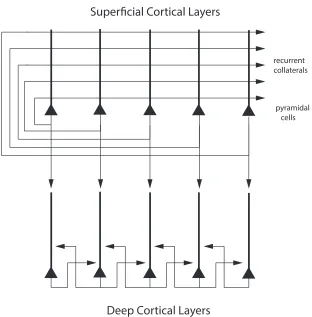
Both the superficial and the deep layers of the cerebral cortex have a highly developed excita-tory recurrent collateral system, with thousands of synapses on the dendrites of each neuron for the recurrent collaterals from nearby neurons (Harris & Shepherd 2015, Rolls 2016, Lefort et al. 2009) (see Fig. 1). Evidence that these recurrent collaterals can support attractor states that help to implement short-term memory, long-term memory, and decision-making has been described (Rolls 2016).
A fundamental question is why there are somewhat separate superficial and deep layers of the cerebral cortex. The advantages include the different outputs that may be appropriate for sending to the next stage of the cortical hierarchy to build higher level representations (with their origin in the superficial layer 2 and 3 pyramidal cells), whereas the deep layer pyramidal cells in layer 5 may provide an output more suitable for driving the often motor-related target systems such as the striatum and in the case of V1 the superior colliculus (Rolls 2016). For example, the representations in the superficial pyramidal cells (L2/L3) may be more sparse than the deep pyramidal cells (L5/L6) (Harris & Shepherd 2015), and Rolls (2016) hypothesizes that this helps the neocortex to increase the memory capacity of what can be stored in discrete autoassociation networks in the superficial layers. The superficial cortical layers are hypothesized to perform the main computationally useful functions of the cerebral neocortex, which involve feedforward operations to form non-linear combinations of the inputs from previous cortical areas utilizing the convergence from stage to stage to construct useful combinations essential for cortical computation, and to implement using the attractor properties of the recurrent collaterals useful functions such as information storage and retrieval (long-term memory, short-term memory, decision-making, etc). According to the hypotheses being developed, these feedforward competitive learning computations performed by the superficial layers are the computationally useful aspects of the design of the neocortex for building new representations (Rolls 2016).
The L5A pyramidal cells have a well-developed recurrent collateral system, and the hy-pothesis has been proposed that the deep layers may operate as a partly separate attractor from that in the superficial layers, for the L2/L3 pyramidal cell dendrites do not descend into the deep layers of the cerebral cortex in which the deep layer neuron recurrent collaterals make their main local connections with nearby layer 5 pyramidal cells (Rolls 2016) (Fig. 1).
1.2.2 The connectivity of the superficial and deep layers of the neocortex
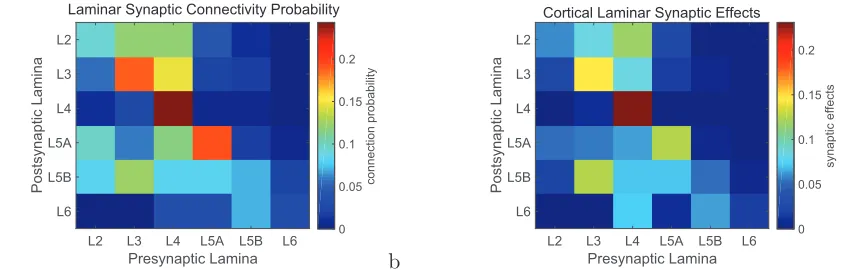
the probability of synaptic connections between pyramidal cells in different laminae by the strength of the synaptic connections between neurons in the different laminae, based on data from Lefort et al. (2009). The quantitative aspects of this connectivity are consistent with the hypothesis that the superficial pyramidal cells with their recurrent collateral connections could form an attractor network, and that the deep pyramidal cells could form a separate attractor network, which receives its inputs from the L3 network in such a way that the L5A network can be driven into activity by the superficial network, and that then the deep network can operate somewhat independently as the coupling between the networks is weaker than the coupling within the networks (Renart, Parga & Rolls 1999a).
Now, this is the case even for rodent whisker barrel somatosensory cortex (Lefort et al. 2009), which is highly dominated by the layer 4 inputs, and in higher cortical areas of primates involved for example in memory the recurrent collateral connections in the superficial and deep layers may be much more highly developed (Elston, Benavides-Piccione, Elston, Zietsch, Defelipe, Manger, Casagrande & Kaas 2006). In this context, it is interesting to note from Fig. 2 that in whisker barrel cortex, layer 4 intralaminar connectivity dominates the intralaminar connectivity, but this will not be the case in most higher cortical areas, for layer 4 become progressively more minimal as one progresses further up a cortical hierarchy (Pandya, Seltzer, Petrides & Cipolloni 2015). It is likely that when frontal and related areas of the cortex involved in memory are investigated, the dominance of the recurrent collateral systems within a cortical layer will become even more apparent, and it will then be of interest to assess quantitatively the relative value of the connectivity from superficial to deep layers compared to that within cortical layers.
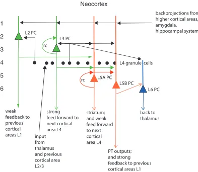
Putting together what is shown in Fig. 2 (based on data from Lefort et al. (2009)) with key findings on cortical connectivity (Pandya et al. 2015, Harris & Shepherd 2015, Markov, Vezoli, Chameau, Falchier, Quilodran, Huissoud, Lamy, Misery, Giroud, Ullman, Barone, Dehay, Knoblauch & Kennedy 2014, Lefort et al. 2009, Hooks et al. 2011, Holmgren et al. 2003, Rockland & Pandya 1979) leads to what is shown in Fig. 1, which is amplified in the following text. Some authors refer to L2 in Fig. 1 as L2/3A; and to L3 as L3B (Harris & Shepherd 2015). The quantitative aspects of the connectivity in higher cortical areas are likely to be much less influenced by L4 than what is shown in Fig. 2, which is for rodent whisker barrel (primary somatosensory) cortex (Lefort et al. 2009).
TheL4 granule cellsreceive strong thalamic inputs, which also reach to a smaller extent neurons in other cortical layers. L4 projects on to neurons in other layers as shown in Fig. 2. L4 becomes progressively smaller up each cortical hierarchy (Pandya et al. 2015), for as one progresses up the hierarchy, the inputs that dominate the processing come more and more from neurons in L3 of the preceding cortical area. L4 has strong onward connections to L3 and L2, and somewhat weaker to neurons in deeper cortical layers (Fig. 2). As shown in Fig. 2 the L4 neurons in whisker barrel cortex have many connections with each other. This may reflect the operation of a L4 attractor network used to help minimize noise and perform constraint satisfaction (Rolls 2016) to produce a population code that best represents the inputs from the sensory receptors associated with a single whisker. In whisker barrel cortex, L6 does not project back to L4, though it does in some other cortical areas (Harris & Shepherd 2015).
L2 receives its inputs from L4 > L3 > L2 (where > should be read as ‘more strongly than’). L2 projects to L5A and L2>L3 and L5B. L2 neurons provide weak cortico-cortical feedback to L1 of the preceding cortical area in a hierarchy.
(Rolls 2016). L3 has strong forward projections to the middle layers of the next layer in the cortical hierarchy, and these are precisely directed to primarily the next cortical area. L3 has strong connections to L5A and L5B pyramidal cells.
L5A has a highly developed recurrent collateral system to other L5A neurons, and this provides the basis for a cortical attractor network in the deep layers of the neocortex (Rolls 2016). Because L5A does not have strong projections to the superficial layers, it could not contribute to and be fully part of any attractor process implemented by the L3 neurons. L5A receives its main inputs from L2, L3, and L4. It has weak forward projections to the middle layers of the next layer in the hierarchy, and these are precisely directed to the next cortical area. L5A neurons have outputs to the striatum (caudate, putamen, and ventral striatum), which is an evolutionarily old region. An interesting hypothesis is that in the evolution of the cortex, the deep layers evolved early in order to provide essential outputs for the cortex; and that the superficial layers developed progressively later to provide for feedforward cortico-cortical computation up the hierarchy as new areas were added in evolution at the end of the existing hierarchy.
L5Bis unlikely to implement an attractor network, as it does not have a high probability of recurrent collateral connections to other L5B neurons (Fig. 2). The main inputs to L5B pyramidal neurons are from L3 >L4 = L5A. (This L5B does receive from an attractor, L3.) L5B has pyramidal tract (PT) outputs, which may be evolutionarily newer than the striatal outputs of L5A. L5B may act as a relay for L3, L4, and L5A (which are both attractors, so it may not need to be an attractor in its own right). L5B is the source of the strong cortico-cortical backprojections, which end mainly in layer 1 of the preceding cortical area, but all backprojections tend to be diffuse in that they project also to earlier cortical areas in the hierarchy (Pandya et al. 2015, Markov et al. 2014).
L6 is cortico-thalamic. Its inputs come from L4 and L5B. So L6 is not strongly influ-enced by an attractor. It may primarily implement a negative feedback to the thalamus, implementing gain control.
The average connectivity between pyramidal cells in mouse whisker barrel cortex is 0.10%, but this is a small column of approximately 300 µm in diameter (Lefort et al. 2009), and in more typical cortex the connectivity may not be restricted by the presence of a barrel de-voted to a single whisker. Indeed, in rat visual and somatosensory neocortex layers L2–L3 the probability of a connection between pyramidal cells in these superficial layers decreases from 0.09 to 0.01 over a radial distance of 25-200 µm (Holmgren et al. 2003). The connections with inhibitory interneurons are somewhat more widely distributed (Holmgren et al. 2003), consis-tent with the hypothesis that the interneurons provide for feedback inhibition to maintain the stability of the excitatory networks and to control the sparseness of the representation, that is, the proportion of the neurons that are active to any one stimulus or event (Rolls 2016).
Further evidence on somewhat separate computations in superficial and deep layers is that different tuning has been found for neurons in superficial vs deep layers of the macaque striate cortex, with the deep layer neurons suggested to be more appropriate for generating eye movements such as vergence eye movements (Bauer & Dow 1991).
1.3 Hypotheses: partly separate attractor networks in superficial and deep layers
The evidence just described and other evidence led to the hypothesis that the deep layers may operate as a partly separate attractor network from that in the superficial layers (Rolls 2016). What computational function might a separate attractor network perform in the deep layers?
1.3.1 Different time courses in the superficial and deep layers
One hypothesis is that an attractor network in the deep layers might have a different time course, with the potential for a shorter time course of firing, consistent with the more bursty firing sometimes reported in the deep layers (Harris & Shepherd 2015), and which may be more suitable for precise temporally accurate motor control (Rolls 2016). The hypothesis is that the deep layers might be temporally faster, as the premium is now on what may sometimes be a requirement for fast but brief output to suddenly drive motor systems when necessary. In contrast, the superficial layers may benefit from slower integration of information, to help build useful new categories, and to allow representations to be influenced by not only the recurrent collaterals, but also by what may be being backprojected from the next cortical stage in the hierarchy (Rolls 2016, Rolls 2012b). This hypothesis is investigated in Experiment 1 by introducing adaptation into the neurons in the deep layer attractor network. The hypothesis that is tested is that the L5A attractor network may have more neuronal adaptation, or synaptic adaptation in its recurrent collaterals, than is the case for L3 neurons, and that this may enable L5A neurons to have shorter periods of attractor-related firing to implement temporally exact motor control; whereas the L3 attractor network with less adaptation in its recurrent collaterals may produce a typically longer time course of its firing, helping to provide a more prolonged input to help the next cortical area learn and to implement processes such as slow learning which are believed to be important in learning transform-invariant representations, and also short-term memory by prolonged firing (Rolls 2016, Rolls 2012b).
1.3.2 Discrete vs spatially continuous attractors in the superficial and deep lay-ers
A second hypothesis is that layer 5A operates as an attractor network, but of a different type to the attractor network in the L3 superficial pyramidal cells. For example, the L3 pyramidal neurons may often need to support discrete attractor states, such as whether it is this object, or that object, especially in the ventral cortical areas involved in ‘what’ representations for visual, auditory, taste, and olfactory stimuli (Rolls 2016). (Discrete representations involve different subsets of neurons firing to represent different objects. The subsets may overlap, but separate objects are represented, without smooth continuity over the representational space (Rolls 2016, Rolls & Treves 2011).) The following proposal follows from the evidence that the pyramidal cells of L5A project to motor structures such as the striatum (Fig. 1).
position in the space can become associated with each other, thus smoothing the transitions through the space by making sure that all neurons relevant to a particular position in the space based on previous experience are recruited into activity.
In this context, it should be noted that networks with associatively modifiable recurrent collateral synapses do not necessarily need to have a positive feedback gain sufficiently high to maintain the activity in a high firing rate attractor state even when there is no input. The network with the structure of an attractor network can nevertheless perform constraint satisfaction, by providing a moderate input from other neurons in the network to add to and smooth whatever inputs are providing the main driving input to the network, which in this case would be a L2/L3 input driving the L5 pyramidal cell firing. This would help to provide a smooth trajectory through the continuous attractor space of movements, without jerks and incompatible motor commands being produced, as described by Rolls (2016).
2
Experiment 1: The effects of adaptation in the deep layers
of the neocortex on the time course of the firing
The faster time course of the deeper layers might be implemented by having relatively fast synaptic or neuronal adaptation (Rolls (2016), cf. Markram et al (2015) who show that adap-tation varies greatly between different classes of cortical neuron). In this experiment, both the superficial and the deep layers were discrete attractor networks, but neuronal adaptation was present in the deep layer attractor network to investigate the hypothesis. A faster time course in deep layers might also be produced by a relatively higher proportion of AMPA or kainate receptors with their short time constant (5–10 ms) in the deep layers, with relatively more NMDA receptors with their relatively long time constants (100 ms) in superficial layers. Consistent with this hypothesis, NMDA receptors are present in relatively higher densities in superficial layers (L2/L3), and kainate receptors in relatively higher densities in deep layers (L5 and L6) of the human fusiform gyrus, a ventral stream visual area involved in face and object processing (Caspers, Palomero-Gallagher, Caspers, Schleicher, Amunts & Zilles 2015). In addition, the pyramidal cells in the deep layers probably have different time constants, for they tend to be large, related in part to the fact that many of their axons have to travel long distances to reach their motor targets and therefore need fast conduction velocities.
2.1 Methods
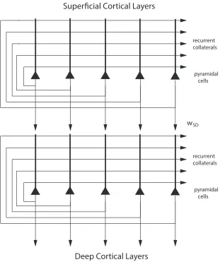
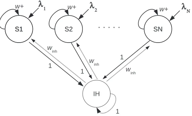
Two attractor networks were implemented as illustrated in Fig. 3. The two networks are connected by synapses from the superficial to the deep layer network with strengthwSD.
The aim is to investigate the operation of the system in a biophysically realistic attractor framework, so that the properties of receptors, synaptic currents and the statistical effects related to the probabilistic spiking of the neurons can be part of the model. We use a minimal architecture, a single attractor or autoassociation network (Hopfield 1982, Amit 1989, Hertz, Krogh & Palmer 1991, Rolls & Treves 1998, Rolls & Deco 2002, Rolls 2008) for each module. A recurrent (attractor) integrate-and-fire network model which includes synaptic channels for AMPA, NMDA and GABAA receptors (Brunel & Wang 2001, Rolls & Deco 2010) was used. The single superficial and the deep discrete attractor networks each contained 800 excita-tory, and 200 inhibitory neurons, which is consistent with the observed proportions of pyra-midal cells and interneurons in the cerebral cortex (Abeles 1991, Braitenberg & Sch¨utz 1991). The connection strengths are adjusted using mean-field analysis (Brunel & Wang 2001, Deco & Rolls 2006, Rolls & Deco 2010, Rolls 2016), so that the excitatory and inhibitory neu-rons exhibit a spontaneous activity of 3 Hz and 9 Hz, respectively (Wilson, O’Scalaidhe & Goldman-Rakic 1994, Koch & Fuster 1989). The recurrent excitation mediated by the AMPA and NMDA receptors is dominated by the NMDA current to avoid instabilities during delay periods (Wang 2002).
The architecture of the cortical network module which is the architecture of both the superficial and the deep attractor networks as illustrated in Fig. 4 has 10 selective pools each with 80 excitatory neurons. The connection weights between the neurons within each pool or population are called the intra-pool connection strengthsw+, which were set to values in the range 1.9–2.2 for the simulations described. All other weights includingwinh were set to 1.
this bias which is present by default arrives at an average spontaneous firing rate of 3 Hz from each external neuron onto each of the 800 synapses for external inputs, consistent with the spontaneous activity observed in the cerebral cortex (Wilson et al. 1994, Rolls & Treves 1998, Rolls 2016).
Both excitatory and inhibitory neurons are represented by a leaky integrate-and-fire model (Tuckwell 1988). The basic state variable of a single model neuron is the membrane potential. It decays in time when the neurons receive no synaptic input down to a resting potential. When synaptic input causes the membrane potential to reach a threshold, a spike is emitted and the neuron is set to the reset potential at which it is kept for the refractory period. The emitted action potential is propagated to the other neurons in the network. The excitatory neurons transmit their action potentials via the glutamatergic receptors AMPA and NMDA which are both modeled by their effect in producing exponentially decaying currents in the postsynaptic neuron. The rise time of the AMPA current is neglected, because it is typically very short (<1 ms). The NMDA channel is modeled with an alpha function including both a rise and a decay term. In addition, the synaptic function of the NMDA current includes a voltage dependence controlled by the extracellular magnesium concentration (Jahr & Stevens 1990). The inhibitory postsynaptic potential is mediated by a GABAA receptor model and is described by a decay term. A detailed mathematical description is provided in the Appendix. A property of cortical neurons is that they tend to adapt with repeated input (Abbott, Varela, Sen & Nelson 1997, Fuhrmann, Markram & Tsodyks 2002). The mechanism is un-derstood as follows. The afterpolarization (AHP) that follows the generation of a spike in a neuron is primarily mediated by two calcium-activated potassium currents, IAHP and the sIAHP(Sah & Faber 2002), which are activated by calcium influx during action potentials. The
IAHP current is mediated by small conductance calcium-activated potassium (SK) channels, and its time course primarily follows cytosolic calcium, rising rapidly after action potentials and decaying with a time constant of 50 to several hundred milliseconds (Sah & Faber 2002). In contrast, the kinetics of the sIAHP are slower, exhibiting a distinct rising phase and de-caying with a time constant of 1–2 s (Sah 1996). A variety of neuromodulators, including acetylcholine (ACh) acting via a muscarinic receptor, noradrenaline, and glutamate acting via G-protein-coupled receptors, suppress the sIAHP and thus reduce spike-frequency adaptation (Nicoll 1988).
When recordings are made from single neurons operating in physiological conditions in the awake behaving monkey, peristimulus time histograms of inferior temporal cortex neurons to visual stimuli show only limited adaptation. There is typically an onset of the neuronal response at 80–100 ms after the stimulus, followed within 50 ms by the highest firing rate. There is after that some reduction in the firing rate, but the firing rate is still typically more than half-maximal 500 ms later (see example in Tovee, Rolls, Treves & Bellis (1993)). Thus under normal physiological conditions, some, but limited, firing rate adaptation can occur.
5.2.
2.2 Results
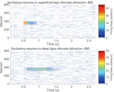
In the first experiment to illustrate the effects of adaptation in the deep discrete attractor network, after 500 ms of spontaneous activity, pool 5 was activated for 100 ms, and its firing stopped within 200 ms, as w+ was set to 1.9 to help the superficial attractor to stop firing relatively soon after stimulus offset (Fig. 5). Through the connection to the deep discrete attractor network with strength wSD = 0.15, pool 5 in the deep attractor started firing, and continued firing for some time with its w+ = 2.2. This demonstrates that the deep network was operating as a discrete attractor network that could maintain its firing for longer than the input from the superficial layers was firing. However, with the neuronal adaptation switched on (with τCa =150 ms and AHP-Ca = 1.0), the deep attractor network did stop firing after approximately 800 ms of activity. If the calcium-implemented neuronal adaptation was switched off, the deep attractor continued to fire indefinitely.
This simulation thus shows that adaptation can set the time course of the deep network when it has been demonstrated to be operating as an attractor (Fig. 5).
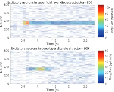
In the second experiment to illustrate the effects of adaptation in the deep discrete attrac-tor network, after 500 ms of spontaneous activity, pool 5 was activated for 200 ms, and its firing continued indefinitely, as w+ was set to 2.05 (Fig. 6). Through the connection to the deep discrete attractor network with strength wSD = 0.1, pool 5 in the deep attractor started firing, and continued firing for some time with its w+ = 2.2. However, with the neuronal adaptation switched on (withτCa =1000 ms and AHP-Ca = 0.4), the deep attractor network did stop firing after approximately 700 ms of activity. If the calcium-implemented neuronal adaptation was switched off, the deep attractor continued to fire indefinitely.
This simulation thus shows that adaptation can set the time course of the deep network even when it continues to receive input from the superficial attractor network (Fig. 6).
Another key issue investigated was the strength of the coupling between the attractor networks in the superficial and deep layers that would allow them to show the partially separate operation described here. For the adaptation effects illustrated in Fig. 6, the coupling term was set to wSD = 0.1, which corresponds to the ratio of the excitatory synaptic weights received by a neuron in the deep layer from the superficial layer to the weights from all recurrent excitatory connections from the other neurons in the deep layers. This value for
net recurrent collateral currents) was 0.21. This higher value forwSDis expected because once a network is in an attractor, it is stable and difficult to perturb (Rolls 2016). This analysis thus helps to provide a framework with which to assess, given the connectivity values shown in Fig. 2, whether the superficial and deep networks are connected so that they can operate as coupled but somewhat independent attractor networks (see Discussion).
3
Experiment 2: A discrete attractor network for the
superfi-cial layers and a continuous attractor network for the deep
layers
In Experiment 2 the aim was to investigate whether the deep and superficial layer recurrent collaterals could implement different types of attractor network and computations. This was investigated with an integrate-and-fire network of a small patch or module or column of neocortex in which the superficial layers were modelled as a fully connected discrete attractor network, which connected with stronger forward than backward connections to the deep layers modelled as an integrate-and-fire continuous attractor network with strong local connectivity between nearby neurons, as illustrated in Fig. 7.
3.1 Method
The superficial layers were modelled as a discrete attractor network as illustrated in Fig. 4. The network is an integrate-and-fire attractor network with npossible attractor states. For the simulations described here there were n=10 orthogonal attractor states in the superficial layer discrete attractor network, each implemented by a population of neurons with strong excitatory connections between the neurons with value w+=2.1 for the NMDA and AMPA synapses. There were always Ns=500 neurons in the module, of which 0.8 were excitatory, and 0.2 were inhibitory. The parameters in the module were set so that the spontaneous firing state with no input applied was stable, and so that only one of its npossible attractor states was active at any time when inputs were applied (Rolls 2016, Rolls & Deco 2010, Deco et al. 2013) (see Appendix).
The deep layer module was modelled as an integrate-and-fire continuous attractor network. The main difference was that the (excitatory) recurrent collaterals connected more strongly to their neighbours than to more distant neurons (see Fig. 7), with a Gaussian function of width
The deep module, the continuous attractor network, operated with similar integrate-and-fire neurons. The inhibition in the continuous attractor network was set to 1.03, and a target parameter that adjusted the equivalent of w+ for the deep network was set to a value that enabled the continuous attractor network to maintain its activity once started (and in the absence of more than spontaneous firing in the superficial network) but with a peak firing rate still in the biological range of less than approximately 100 spikes/s (Rolls & Treves 2011, Rolls 2016).
It is noted that this type of continuous attractor network is described as having metric connectivity, in that the recurrent connections between the pyramidal cells are short range (Roudi & Treves 2008). This can be set up by self-organising learning, as illustrated by Rolls (2016). A different scenario for a continuous attractor network is when the connectivity is global, and the continuous attractor network is set up by learning which of the neurons with a Gaussian tuning profile are close together in the space being represented while the agent or animal traverses the space repeatedly (Rolls 2016).
An important difference in these discrete and continuous attractor networks is in the learning. In a discrete attractor network it is assumed that a random set of neurons is caused to fire by the inputs being received. Competitive learning may be involved in this process (Rolls 2016). The recurrent collateral connections between the neurons then show associative (Hebbian) synaptic modification. The set of currently active neurons thereby form a discrete attractor, as described by Rolls (2016). A large number of independent representations can be set up in this way. In contrast, in a continuous attractor network, neurons that are nearby in a space tend to excite each other depending on their distance from each other in the space. One way in which such firing might be set up is if the input being received is in some continuous space, such as a space of head direction, or spatial view, or movements being made in 3D space. In this case, Hebbian synaptic modification allows the continuous space to be learned by the continuous attractor network, and near points in the space need not be represented by nearby neurons. Another way in which such continuous representations can be set up is by short-range recurrent collaterals, which, because they are short range and their density falls off with distance across the cortex, tend to make nearby neurons in the cortex have activity to similar stimuli. This is how topographic maps can be formed in the cortex, with an example of such a map being that in the primary visual cortex. These concepts are described in more detail by Rolls (2016). For the present work, which of these two methods is used to set up the continuous attractor network does not matter in principle, but in practice we set up the continuous attractor network by setting up the recurrent collaterals to have a strength of connection to neighbouring pyramidal cells that falls off as a function of distance between the pyramidal cells, which is a property of neocortex (Holmgren et al. 2003).
only to start the deep attractor, after which the nature of the drift was explored without any further input from the superficial network. As was the case for the superficial network, the neurons in the deep network always had an external Poisson input to each of 800 synapses on each neuron set to a default external spontaneous rate of 3 spikes/s on every one of these 800 synapses.
The stability analyses were performed as follows. The deep module continuous attractor was set up as a ring attractor, that is, the end of the excitatory firing rate array was connected back to the start with the local recurrent collateral connections. There were 10 sectors in the ring attractor, in that each of the ten superficial discrete attractors was connected to one tenth of the excitatory neurons in the deep attractor. The amount of drift was measured by the number of the 10 sectors that the centre of gravity of the bubble of activity drifted in 12 s (or by the number of neurons over which the drift occurs). As will be shown, the drift was typically less than the width of one of the 10 sectors in the ring attractor. Simulations were performed with different numbers of neurons in the deep module, to investigate how the size of the continuous attractor and therefore the finite size noise influenced the drift and stability. In addition to the total drift over 12 s, a second measure was the short-term movement, again measured in sectors or in neurons, that occurred between the centre of gravity of the bubble measured every 100 ms.
During operation, one attractor pool in the superficial module received an increased input for 1000 ms starting after an initial 500 ms period of spontaneous firing. That started firing in the deep module.
3.2 A hypothesis: adaptation must be minimal in a continuous attractor network
It is hypothesized here that any adaptation in a continuous attractor network will impair its stability, because when neurons in the packet of activity adapt, the lower firing neurons at the edge of the activity packet will be less adapted, and the packet of activity will drift towards the less adapted neurons. This is hypothesized here to be an important constraint on the operation of continuous attractor networks in the brain. An implication and prediction is that states in which adaptation is more likely to occur, including drowsiness when cholinergic neuronal firing may be reduced, or the use of a cholinergic blocker such as scopolamine, may impair tasks that involve idiothetic (i.e. self-motion) update of position such as head direction, eye position, how far one has travelled, etc. Cholinergic projections from the basal forebrain are important in minimizing cortical adaptation, and the basal forebrain neurons are activated by rewarding, punishing, and novel stimuli (Rolls & Deco 2015b, Rolls 2016, Rolls 2014, Rolls, Burton & Mora 1976, Burton, Rolls & Mora 1976, Mora, Rolls & Burton 1976, Rolls, Sanghera & Roper-Hall 1979, Wilson & Rolls 1990b, Wilson & Rolls 1990a, Wilson & Rolls 1990c), all of which help to maintain a non-adapted cortex. (Scopolamine is frequently prescribed for travel sickness, and it is suggested might operate by reducing the stability of continuous attractor networks, so that there would be less discrepancy between them and visual motion cues, in that the continuous attractor networks may be more easily driven by visual inputs.)
macaque (Tovee, Rolls, Treves & Bellis 1993). In particular, [Ca2+] is initially set to be 0
µM, τCa = 300 ms, α = 0.002, VK =−80 mV and gAHP=200 nS unless otherwise specified. (We note that there are a number of other biological mechanisms that might implement the slow transitions from one attractor state to another, some investigated by Deco & Rolls (2005), and that we use the spike frequency adaptation mechanism to illustrate the principles of operation of the networks.)
3.3 Results
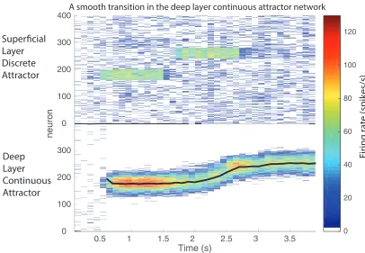
3.3.1 Smooth transitions in the Deep Network Continuous Attractor Module
If the deep network made a transition from one position corresponding to one of the superficial pools, to another position corresponding to another superficial pool, the transition under some circumstances of the deep pool could be continuous. This is illustrated in Fig. 8, in which a smooth transition occurred in the continuous attractor network when the superficial attractor network jumped from pool 3 (neurons 80 to 120 given that there were 400 excitatory neurons divided into 10 pools) to pool 5 (neurons 160–200). This was found to occur primarily when the width of the bubble spanned the first and second parts of the space over which a transition had to be made.
This may be helpful biologically, by smoothing transitions between nearby states.
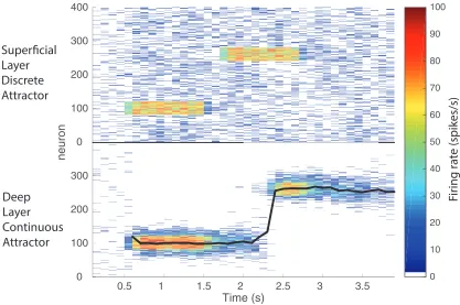
When the transition being driven by the superficial network was larger than the width of the bubble, the bubble simply stopped in the first position, and started in the new position, with what appeared to be an abrupt jump. This is illustrated in Fig. 9, when the superficial network jumped from pool 3 to pool 7. This resulted in a jump in the deep continuous attractor network. This may be biologically plausible, for it may not be appropriate for the deep network to transition through all the intermediate positions when two distant positions for the superficial network are successively active.
A third scenario occurs when the deep continuous attractor network has entered a region of attraction, i.e. firing has started. The deep continuous attractor is then more stable than when its neurons are just firing at a spontaneous rate. Under these conditions, only a strong input from the superficial attractor will move the deep attractor to a new position. This may provide some form of noise tolerance for the deep, continuous attractor, network. The higher the firing rate of the continuous attractor, the more resistant it is to being perturbed by an external input.
3.3.2 Stability of the integrate-and-fire stochastic spiking continuous attractor network
The stability of the integrate-and-fire continuous attractor network was measured in a 12 s period starting after time=2 s in a simulation during which the bubble of activity was maintained. The start time was thus after the end of the period in which the superficial attractor had been active, as illustrated in Fig. 10. In this case, there were only 200 excitatory neurons in the deep continuous attractor network, and both short-term noise due to the statistical fluctuation in the numbers of spikes in the different neurons was evident, as well as long-term drift.
attractor had been removed. The measure was the absolute value of the number of neurons over which the centre of gravity of the bubble had drifted in a 12 s period. Considerable stability was evident, as illustrated in Fig. 11. Indeed, the typical drift over 12 s was rather small (a drift of between 5 and 10 neurons, with standard deviation of approximately 5). There was no significant effect of N on the long-term drift. Although there may be short-term statistical fluctuations with the bubble moving left or right in a short time period in the order of 100 ms, these short term drifts largely cancel out over long periods.
It is notable in Fig. 11 that there was relatively little effect of the number of excitatory neurons N in the continuous attractor network on the number of neurons over which the packet of activity fluctuated or drifted. The implication is that if the continuous attractor ring represents the whole of a space, then having more neurons in the ring continuous attractor results in more stability of the representation expressed as the fraction of the ring (and of the whole space) over which the centre of gravity moves.
The factors that lead to the stability of even relatively small continuous attractor networks with spiking neurons are considered in the Discussion.
3.3.3 Effects of adaptation on the stability of the deep layer continuous attractor
Both synaptic and neuronal adaptation can occur, and can be modelled (Deco & Rolls 2005). The hypothesis proposed is that adaptation would affect the stability of the continuous at-tractor network, for as neurons fire less because of adaptation, other neurons in the fringes of the continuous attractor bubble with lower firing rates but still being activated by the local recurrent collaterals would be less adapted, so would start to fire more than neurons at the centre of the activity packet. This was expected to cause the deep continuous attractor network to drift continuously across the space being represented.
This hypothesis was tested by implementing neuronal firing rate adaptation as described in Section 5.2. This had the effect of causing the packet of activity to become unstable, and to drift continuously across the space being represented, as illustrated in Fig. 12. In this simulation τCa = 300 ms, and the target parameter for the deep w+ was 3.3. On different trials with different random seeds the drift was in different directions, but once started, continued in the same direction, right round the ring attractor if left for sufficiently long. Any adaptation can thus impair the stability of a continuous attractor network.
4
Discussion
be useful in the training of the next layers up in the hierarchy, using for example slow learning (Rolls 2012b, Rolls 2016).
A key issue in understanding whether the superficial and deep layers of the neocortex could operate as separate attractors with the superficial influencing the deep attractor networks but not fully determining their states is the nature of the connectivity from the superficial layers to the deep layers. One key condition is that the number of connections from neurons in the the superficial layers to any single neuron in the deep layers must be in the order of the the number of connections onto any one neuron in the superficial layers from the other neurons in the superficial layers via the recurrent collaterals. The quantitative argument is the same as for the number of backprojections in the cerebral cortex onto any one neuron compared to the number of connections between hippocampal CA3 neurons, and arises because if one can represent a certain number of memory states with the recurrent collaterals, then one needs to be able to transmit the same number of states (Treves & Rolls 1994, Rolls 2016). This condition appears to be approximately satisfied by the number of connections from L3 to each L5 neuron relative to the number of recurrent collaterals onto any one L3 neuron from other L3 neurons (Fig. 2a).
A second key condition is that the strength of the synaptic connections from the superficial layers to the deep layers must be sufficiently strong that these connections can start up an attractor state in the deep layers, or shift it from one attractor state to another. It is shown in Section 2.2 that for these effects, wSD needs to be in the range of approximately 0.1–1.0, with the corresponding current ratios of forward to recurrent currents greater than 0.2. At the same time, some independence of operation of the two networks was found withwSD=0.5 and the current ratio 0.74, in that the deep but not the superficial network could then adapt out to produce a burst of firing in the deep layers but with a longer period of firing being maintained in the superficial layers. The calculated currents between neurons in different layers illustrated in Fig. 2b are fully consistent with the results described in the present investigations. (We note that the issue of whether the connectivity is diluted in each of the superficial and deep attractor networks is not the issue here. Dilution helps by reducing the distortion of the basins of attraction that would be produced if by chance there were many pairs of neurons with two or more recurrent collateral synapses between any pair of neurons (Rolls 2012a). The issue here is of the ratio of the connectivity between and within coupled attractor networks (Rolls 2016)).
deep layers of the neocortex.
The results presented here for Experiment 2 show how the deep layers might perform a different type of computation to the superficial layers. In the example used to illustrate this potential principle of operation of the cerebral cortex, a continuous attractor network implemented by local recurrent collateral synaptic connections in the deep layers could enable smooth changes from one representation to another when the representations are relatively close in the space. It is also shown that in the integrate-and-fire continuous attractor network with neurons that fire stochastically the packet of neuronal firing is relatively stable. This may be because the short-term statistical fluctuations caused by the random spiking times of the neurons for a given mean rate tend to cancel out over periods of 100 ms or more. It is also shown that any neuronal adaptation would cause drift across the space being represented, with the implication that some continuous attractor networks in the brain should have little neuronal, or synaptic, adaptation, in order to provide for path integration (Rolls 2016). On the other hand, in some parts of the cortex, some adaptation and therefore drift might have evolved as a mechanism for forward movement, rhythm, music, song and speech (Rolls & Deco 2015a).
In relation to the stability of the continuous attractor network implemented with integrate-and-fire neurons, it was found that the long-term drift did not alter significantly asNincreased (Fig. 11). An implication is that if a ring continuous attractor had to represent a certain physical space, say 360 degrees of space, then the net effect of having more neurons (i.e. increasing N) would mean less drift per unit of physical space. In effect, the measure of drift expressed as the proportion of the physical space being represented decreases as the size of the continuous attractor network, N, increases.
One possibility was that the drift in the continuous attractor network might have been greater with small networks, for then the statistical fluctuations in the firing rates would be larger. In discrete attractor networks, this variability can influence the decision-making (Deco & Rolls 2006, Rolls, Grabenhorst & Deco 2010, Rolls 2016), and has been observed in continuous attractor networks (Cerasti & Treves 2013). However, in the present simulations there was not more drift in the smaller continuous attractor networks than the large networks (Fig. 11). The reason for our finding is that we kept the width of the bubble of activity constant when we increased the number of neurons in the network. Thus the number of neurons active in our simulations, and generating the statistical fluctuations in firing rates, was constant when we increased the size of the network, and that is the reason we propose why the stability measured by the drift did not alter significantly when we increased the size on the network. In contrast, Cerasti & Treves (2013) kept the spatial geometry of their inputs constant when they increased the size of the network, so that more neurons were allocated to a packet of activity as the number of neurons in the network was increased. We hypothesize that it was because in their simulations more neurons were active as the size of the network increased that they observed a reduction of noise, evident as drift, as they increased the size of the network.
discrete (for objects) and continuous (for scenes and places) representations (Rolls, Stringer & Trappenberg 2002, Rolls 2016, Rolls 2017). This would be important in for example a hippocampal memory system (Rolls et al. 2002, Rolls 2016, Rolls 2017). In so far as the hippocampal system involves associations between discrete objects and continuous spaces, we note that it would not operate well as a continuous attractor for spatial navigation, because the space would be distorted by the discrete object representations. A second scenario is that if there are more neurons in a continuous attractor network, then the number of places or scenes or maps might remain constant, with the consequence that there would then be more neurons in each packet of activity, which would reduce the drift. That is the situation investigated by Cerasti & Treves (2013). We note that even with the quite small networks investigated here, stability over 12 s was not a major issue, and so we believe that the ability to represent more locations, rather than to increase stability, is likely to be more biologically important.
In terms of physics, factors that influence the stability of a continuous attractor network include the following. The first effect is the statistical fluctuations in the firing rate referred to as “fast noise” (Cerasti & Treves 2013). This shows finite size effects, with more noise (or fluctuations) of the firing rate that may produce a drift in activity of the population of neurons present in small networks. This can increase the drift in a continuous attractor network, or lead to more noisy decision-making, memory retrieval, etc in a discrete attractor network (Rolls & Deco 2010, Deco, Rolls, Albantakis & Romo 2013, Rolls 2016). The second effect is the presence of “slow” or “quenched” noise which refers to the fact that with small
N, the synaptic weights in the continuous attractor network have small discontinuities that result in “holes” in the attractor landscape, and these tend to restrict the free movement of the packet of activity whenN is relatively small. This effect would tend to reduce drift in the continuous attractor network with small N. The slow and fast noise can thus operate in opposite directions to influence the stability of a continuous attractor network. The fast noise may be the more important factor, to judge from the results of Cerasti & Treves (2013).
Continuous attractors (in the deep layers) may be especially useful for cortical areas that represent low-dimensional spaces (such as motor areas), for then the continuity of output may help to produce smooth movements. The essence of a continuous attractor is that it can be learned when there is a fixed trajectory through the firing rate state space that is repeated frequently. This might arise for example if three movements regularly followed each other. If running in a 2-dimensional environment occurred, then grid cells might arise in this low-dimensional space with the hexagonal arrangement reflecting the efficient packing possible in this low-dimensional space (Kropff & Treves 2008, Stella & Treves 2015). On the other hand, in regions such as the high order visual cortical areas including the inferior temporal visual cortex where neurons represent a large number of relatively separate objects, faces, etc (Rolls 2012b, Rolls 2016), a fixed order trajectory through this high dimensional state space is unlikely to occur naturally. (That is, 1000 objects are unlikely to be presented in the same sequence regularly!) Thus in high dimensional spaces the utility of some continuity of repre-sentation such as that produced by a continuous attractor network in the deep cortical layers is less clear. However, even in these areas, there may be some similarity structure between stimuli, with some objects more similar to each other than other objects. In this situation, some continuity in the representation may be useful, for then a new object intermediate be-tween the two similar objects can produce an appropriate output correctly mapped into the space without any further learning.
advantage just described of enabling new objects to be placed correctly in a space with some continuities. Such a topographic map (described further by Rolls (2016)) need not be capable of sustained activity which is generally a property of attractor networks. But such a continuous map, perhaps more realised in the deep cortical layers, might still have the desirable property of providing a continuous representation, so that any incoming stimulus not actually seen before can be placed at the correct place in the space being represented.
Indeed, the superficial layers might have in part the properties of a discrete attractor network using the recurrent collaterals; but also might have some mixed continuous properties because of the fact that the recurrent collaterals in the neocortex are relatively short-range, spreading approximately 2 mm. In this scenario, the deep layers might implement a further move towards a continuous attractor, a ‘second stage’.
However, for the feedforward processing from stage to stage in a neocortical hierarchy, discrete representations may be useful, so as not to throw away information about exactly which stimulus is present. The connectivity of the superficial layers seems to provide for this, with the input to any one stage being received predominantly into layer 4 and the superficial layers 2 and 3, which in turn project forward to the superficial layers of the next cortical area in the hierarchy (Rolls 2016).
In this scenario, how might more continuous representations in the deep layers be com-putationally useful, apart from facilitating smooth movements and trajectories through state spaces? One interesting possibility is that in language production, in which syntactic role may be encoded in a fixed order such as subject-verb-object, a continuous attractor network for this trajectory through the state space (Rolls & Deco 2015a) might be implemented in the deep cortical layers. It may be more likely that this particular sequence is encoded in the deep layers, for this may be more biologically plausible than that the order is implemented by the feedforward projections between connected cortical areas within a speech production region such as Broca’s area (Rolls & Deco 2015a). Another possibility is that phoneme production in cortical motor areas (Bouchard, Mesgarani, Johnson & Chang 2013) might be implemented in deep layer attractor networks (A.Treves, personal communication). Another possibility is that for the cortico-cortical backprojections, which originate predominantly in primates from the deep layer pyramidal cells in especially layer 5 (Rolls 2016, Pandya et al. 2015), a more continuous representation, possibly less sparse, may be useful, for then the top-down modu-lation of attention and of cognition would then bias on all the neurons in a preceding cortical area in the hierarchy that might be being activated by a particular discrete incoming bottom-up stimulus. This is a computational argument for the backprojections, from mainly the deep layers of the cortex, having a more continuous, and probably less sparse, representation than the superficial layers of the neocortex (Rolls 2016).
In this research, we have explored hypotheses about possible differences in the computa-tions performed by the superficial and deep layers of the neocortex. We have demonstrated some possible principles of operation of the deep layers of the neocortex if they implement, in part, continuous attractor networks. These principles include being able to produce smooth outputs, and producing continuous outputs less sparse than those of the superficial layers which may be useful for top-down backprojected information for attentional and cognitive modulation. (The sparser representations that may be more evident in the superficial layers may be more useful for storing large numbers of different, discrete, representations in a dis-crete attractor network, and for looking up particular objects using forward cortico-cortical processing in a hierarchy.) Nevertheless there are other computational advantages of having somewhat computationally different superficial and deep layers of the neocortex, and we re-gard the present work as an exploration of possibilities and possible implementations, rather than proving that the deep layers have different functions computationally to the superficial layers. Moreover, we note that the hypotheses that are explored here may not be compatible with each other in an implementation of the neocortex, as each hypothesis requires different parameters, especially with respect to adaptation.
Acknowledgements
5
Appendix
5.1 Implementation of neural and synaptic dynamics
We use the mathematical formulation of the integrate-and-fire neurons and synaptic currents described by Brunel & Wang (2001). Here we provide a brief summary of this framework.
The dynamics of the sub-threshold membrane potential V of a neuron are given by the equation:
Cm
dV(t)
dt =−gm(V(t)−VL)−Isyn(t), (1)
Both excitatory and inhibitory neurons have a resting potential VL = −70mV, a firing thresholdVthr =−50mV and a reset potential Vreset=−55mV. The membrane parameters are different for both types of neurons: Excitatory (Inhibitory) neurons are modeled with a membrane capacitance Cm = 0.5nF (0.2nF), a leak conductance gm = 25nS (20nS), a membrane time constant τm = 20ms (10ms), and a refractory period tref = 2ms (1ms). Values are extracted from McCormick, Connors, Lighthall & Prince (1985).
When the threshold membrane potential Vthr is reached, the neuron is set to the reset potential Vreset at which it is kept for a refractory period τref and the action potential is propagated to the other neurons.
The network is fully connected with NE = 800 excitatory neurons and NI = 200 in-hibitory neurons, which is consistent with the observed proportions of the pyramidal neurons and interneurons in the cerebral cortex (Braitenberg & Sch¨utz 1991, Abeles 1991). The synaptic current impinging on each neuron is given by the sum of recurrent excitatory cur-rents (IAM P A,rec and IN M DA,rec), the external excitatory current(IAM P A,ext) the inhibitory current (IGABA):
Isyn(t) =IAM P A,ext(t) +IAM P A,rec(t) +IN M DA,rec(t) +IGABA(t). (2)
The recurrent excitation is mediated by the AMPA and NMDA receptors, inhibition by GABA receptors. In addition, the neurons are exposed to external Poisson input spike trains mediated by AMPA receptors at a rate of 2.4 kHz. These can be viewed as originating from Next= 800 external neurons at an average rate of 3 Hz per neuron, consistent with the spontaneous activity observed in the cerebral cortex (Wilson et al. 1994, Rolls & Treves 1998). The currents are defined by:
IAM P A,ext(t) = gAM P A,ext(V(t)−VE) NXext
j=1
sAM P A,extj (t) (3)
IAM P A,rec(t) = gAM P A,rec(V(t)−VE) NE
X
j=1
wjiAM P AsAM P A,recj (t) (4)
IN M DA,rec(t) =
gN M DA(V(t)−VE) 1 + [M g++]exp(
−0.062V(t))/3.57 × NE
X
j=1
wjiN M DAsN M DAj (t) (5)
IGABA(t) = gGABA(V(t)−VI) NI
X
j=1
whereVE = 0 mV, VI =−70 mV, wj are the synaptic weights, sj’s the fractions of open channels for the different receptors and g’s the synaptic conductances for the different chan-nels. The NMDA synaptic current depends on the membrane potential and the extracellular concentration of Magnesium ([M g++] = 1 mM (Jahr & Stevens 1990)). The values for the synaptic conductances for excitatory neurons aregAM P A,ext= 2.08 nS,gAM P A,rec= 0.104 nS,
gN M DA = 0.327 nS and gGABA= 1,25 nS ; and for inhibitory neuronsgAM P A,ext= 1.62 nS,
gAM P A,rec= 0.081 nS,gN M DA = 0.258 nS andgGABA = 0.973 nS. These values are obtained from the ones used by Brunel & Wang (2001) by correcting for the different numbers of neu-rons. The conductances were calculated so that in an unstructured network the excitatory neurons have a spontaneous spiking rate of 3 Hz and the inhibitory neurons a spontaneous rate of 9 Hz. The fractions of open channels are described by:
dsAM P A,extj (t)
dt = −
sAM P A,extj (t)
τAM P A
+X
k
δ(t−tkj) (7)
dsAM P A,recj (t)
dt = −
sAM P A,recj (t)
τAM P A
+X
k
δ(t−tkj) (8)
dsN M DA j (t)
dt = −
sN M DA j (t)
τN M DA,decay
+αxj(t)(1−sN M DAj (t)) (9)
dxj(t)
dt = −
xj(t)
τN M DA,rise
+X
k
δ(t−tkj) (10)
dsGABA
j (t)
dt = −
sGABA j (t)
τGABA
+X
k
δ(t−tkj), (11)
where τN M DA,decay = 100 ms is the decay time for NMDA synapses, τAM P A = 2 ms for AMPA synapses (Hestrin, Sah & Nicoll 1990, Spruston, Jonas & Sakmann 1995) and
τGABA= 10 ms for GABA synapses (Salin & Prince 1996, Xiang, Huguenard & Prince 1998);
τN M DA,rise= 2 ms is the rise time for NMDA synapses (the rise times for AMPA and GABA are neglected because they are typically very short) and α = 0.5 ms−1. The sums over k represent a sum over spikes formulated as δ-Peaks δ(t) emitted by presynaptic neuron j at time tkj.
The equations were integrated numerically using a second order Runge-Kutta method with step size 0.02 ms. The Mersenne Twister algorithm was used as random number generator for the external Poisson spike trains.
5.2 Calcium-dependent spike frequency adaptation mechanism
A specific implementation of the spike-frequency adaptation mechanism using Ca++-activated K+ hyper-polarizing currents (Liu & Wang 2001) is described next, and was used by Deco & Rolls (2005). We assume that the intrinsic gating of K+ After-Hyper-Polarizing current (IAHP) is fast, and therefore its slow activation is due to the kinetics of the cytoplasmic Ca2+ concentration. This can be introduced in the model by adding an extra current term in the integrate-and-fire model, i.e. by addingIAHPon the right hand of equation 12, which describes the evolution of the subthreshold membrane potential V(t) of each neuron:
Cm
dV(t)
whereIsyn(t) is the total synaptic current flow into the cell, VL is the resting potential, Cm is the membrane capacitance, andgm is the membrane conductance. The extra current term that is introduced into this equation is as follows:
IAHP=−gAHP[Ca2+](V(t)−VK) (13)
whereVK is the reversal potential of the potassium channel. Further, each action potential generates a small amount (α) of calcium influx, so that IAHP is incremented accordingly. Between spikes the [Ca2+] dynamics is modelled as a leaky integrator with a decay constant
τCa. Hence, the calcium dynamics can be described by following system of equations:
d[Ca2+]
dt =−
[Ca2+]
τCa
(14)
IfV(t) =θ, then [Ca2+] = [Ca2+] +α andV =Vreset, and these are coupled to the equations of the neural dynamics provided here and elsewhere (Rolls & Deco 2010, Rolls 2016). The [Ca2+] is initially set to be 0 µM, τ
Ca = 300 ms,α = 0.002, VK =−80 mV and gAHP=0–40 nS. gAHP = 40 nS simulates the effect of high levels of acetylcholine produced alertness and attention, and gAHP= 0 nS simulates the effect of low levels of acetylcholine in normal aging (Rolls & Deco 2015b).
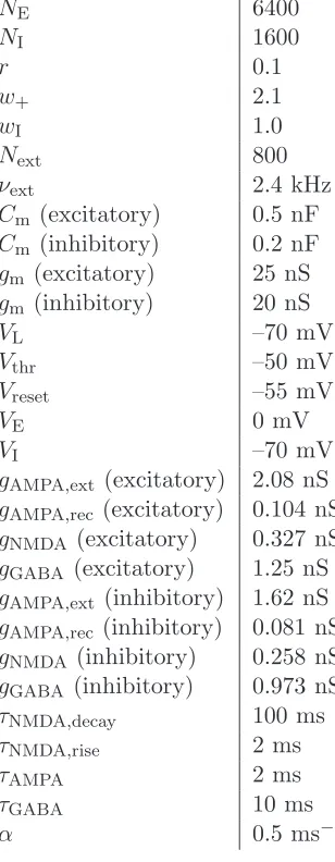
5.3 The model parameters used in the simulations
Table 1: Parameters used for each module in the integrate-and-fire simulations
NE 6400
NI 1600
r 0.1
w+ 2.1
wI 1.0
Next 800
νext 2.4 kHz
Cm (excitatory) 0.5 nF
Cm (inhibitory) 0.2 nF
gm (excitatory) 25 nS
gm (inhibitory) 20 nS
VL –70 mV
Vthr –50 mV
Vreset –55 mV
VE 0 mV
VI –70 mV
gAMPA,ext (excitatory) 2.08 nS
gAMPA,rec (excitatory) 0.104 nS
gNMDA (excitatory) 0.327 nS
gGABA (excitatory) 1.25 nS
gAMPA,ext (inhibitory) 1.62 nS
gAMPA,rec (inhibitory) 0.081 nS
gNMDA (inhibitory) 0.258 nS
gGABA (inhibitory) 0.973 nS
τNMDA,decay 100 ms
τNMDA,rise 2 ms
τAMPA 2 ms
τGABA 10 ms
References
Abbott, L. F., Varela, J. A., Sen, K. & Nelson, S. B. (1997). Synaptic depression and cortical gain control, Science275: 220–224.
Abeles, A. (1991). Corticonics, Cambridge University Press, New York.
Amit, D. J. (1989). Modeling Brain Function. The World of Attractor Neural Networks., Cambridge University Press, Cambridge.
Battaglia, F. P. & Treves, A. (1998). Attractor neural networks storing multiple space repre-sentations: a model for hippocampal place fields,Physical Review E 58: 7738–7753.
Bauer, R. & Dow, B. M. (1991). Local and global principles of striate cortical organization: an advanced model,Biol Cybern 64(6): 477–83.
Bouchard, K. E., Mesgarani, N., Johnson, K. & Chang, E. F. (2013). Functional organization of human sensorimotor cortex for speech articulation, Nature495(7441): 327–32.
Braitenberg, V. & Sch¨utz, A. (1991). Anatomy of the Cortex, Springer Verlag, Berlin.
Brown, D. A., G¨ahwiler, B. H., Griffith, W. H. & Halliwell, J. V. (1990). Membrane currents in hippocampal neurons,Progress in Brain Research 83: 141–160.
Brunel, N. & Wang, X. J. (2001). Effects of neuromodulation in a cortical network model of object working memory dominated by recurrent inhibition,Journal of Computational Neuroscience 11: 63–85.
Burton, M. J., Rolls, E. T. & Mora, F. (1976). Effects of hunger on the responses of neurones in the lateral hypothalamus to the sight and taste of food,Experimental Neurology51: 668– 677.
Caspers, J., Palomero-Gallagher, N., Caspers, S., Schleicher, A., Amunts, K. & Zilles, K. (2015). Receptor architecture of visual areas in the face and word-form recognition region of the posterior fusiform gyrus,Brain Struct Funct 220(1): 205–19.
Cerasti, E. & Treves, A. (2013). The spatial representations acquired in CA3 by self-organizing recurrent connections, Frontiers in Cellular Neuroscience7: 112.
Deco, G. & Rolls, E. T. (2005). Sequential memory: a putative neural and synaptic dynamical mechanism, Journal of Cognitive Neuroscience17: 294–307.
Deco, G. & Rolls, E. T. (2006). A neurophysiological model of decision-making and Weber’s law, European Journal of Neuroscience24: 901–916.
Deco, G., Rolls, E. T., Albantakis, L. & Romo, R. (2013). Brain mechanisms for perceptual and reward-related decision-making, Progress in Neurobiology103: 194–213.
Fuhrmann, G., Markram, H. & Tsodyks, M. (2002). Spike frequency adaptation and neocor-tical rhythms, Journal of Neurophysiology88: 761–770.
Goldman-Rakic, P. (1996). The prefrontal landscape: implications of functional architecture for understanding human mentation and the central executive, Philosophical Transac-tions of the Royal Society London B 351: 1445–1453.
Harris, K. D. & Shepherd, G. M. (2015). The neocortical circuit: themes and variations,
Nature Neuroscience 18: 170–181.
Hertz, J., Krogh, A. & Palmer, R. G. (1991). Introduction to the Theory of Neural Compu-tation, Addison Wesley, Wokingham, U.K.
Hestrin, S., Sah, P. & Nicoll, R. (1990). Mechanisms generating the time course of dual component excitatory synaptic currents recorded in hippocampal slices, Neuron5: 247– 253.
Holmgren, C., Harkany, T., Svennenfors, B. & Zilberter, Y. (2003). Pyramidal cell communi-cation within local networks in layer 2/3 of rat neocortex, J Physiol551(Pt 1): 139–53.
Hooks, B. M., Hires, S. A., Zhang, Y. X., Huber, D., Petreanu, L., Svoboda, K. & Shepherd, G. M. (2011). Laminar analysis of excitatory local circuits in vibrissal motor and sensory cortical areas, PLoS Biol9(1): e1000572.
Hopfield, J. J. (1982). Neural networks and physical systems with emergent collective com-putational abilities, Proc. Nat. Acad. Sci. USA79: 2554–2558.
Jahr, C. & Stevens, C. (1990). Voltage dependence of NMDA-activated macroscopic conduc-tances predicted by single-channel kinetics, Journal of Neuroscience10: 3178–3182.
Koch, K. W. & Fuster, J. M. (1989). Unit activity in monkey parietal cortex related to haptic perception and temporary memory, Experimental Brain Research76: 292–306.
Kropff, E. & Treves, A. (2008). The emergence of grid cells: Intelligent design or just adap-tation?, Hippocampus 18: 1256–1269.
Lanthorn, T., Storm, J. & Andersen, P. (1984). Current-to-frequency transduction in CA1 hippocampal pyramidal cells: slow prepotentials dominate the primary range firing,
Experimental Brain Research 53: 431–443.
Lefort, S., Tomm, C., Floyd Sarria, J. C. & Petersen, C. C. (2009). The excitatory neuronal network of the c2 barrel column in mouse primary somatosensory cortex,Neuron61: 301– 16.
Liu, Y. & Wang, X.-J. (2001). Spike-frequency adaptation of a generalized leaky integrate-and-fire model neuron,Journal of Computational Neuroscience 10: 25–45.
Markram, H., Muller, E., Ramaswamy, S., Reimann, M. W., Abdellah, M., Sanchez, C. A., Ailamaki, A., Alonso-Nanclares, L., Antille, N., Arsever, S., Kahou, G. A., Berger, T. K., Bilgili, A., Buncic, N., Chalimourda, A., Chindemi, G., Courcol, J. D., Delalon-dre, F., Delattre, V., Druckmann, S., Dumusc, R., Dynes, J., Eilemann, S., Gal, E., Gevaert, M. E., Ghobril, J. P., Gidon, A., Graham, J. W., Gupta, A., Haenel, V., Hay, E., Heinis, T., Hernando, J. B., Hines, M., Kanari, L., Keller, D., Kenyon, J., Khazen, G., Kim, Y., King, J. G., Kisvarday, Z., Kumbhar, P., Lasserre, S., Le Be, J. V., Magalhaes, B. R., Merchan-Perez, A., Meystre, J., Morrice, B. R., Muller, J., Munoz-Cespedes, A., Muralidhar, S., Muthurasa, K., Nachbaur, D., Newton, T. H., Nolte, M., Ovcharenko, A., Palacios, J., Pastor, L., Perin, R., Ranjan, R., Riachi, I., Rodriguez, J. R., Riquelme, J. L., Rossert, C., Sfyrakis, K., Shi, Y., Shillcock, J. C., Silberberg, G., Silva, R., Tauheed, F., Telefont, M., Toledo-Rodriguez, M., Trankler, T., Van Geit, W., Diaz, J. V., Walker, R., Wang, Y., Zaninetta, S. M., DeFelipe, J., Hill, S. L., Segev, I. & Schurmann, F. (2015). Reconstruction and simulation of neocortical microcircuitry, Cell 163(2): 456–92.
Marlin, T. E. (2000). Process Control: Designing Processes and Control Systems for Dynamic Performance, McGraw-Hill, Boston. http://pc-textbook.mcmaster.ca/.
Mason, A. & Larkman, A. (1990). Correlations between morphology and electrophysiology of pyramidal neurones in slices of rat visual cortex. I. Electrophysiology, Journal of Neuroscience 10: 1415–1428.
McCormick, D., Connors, B., Lighthall, J. & Prince, D. (1985). Comparative electrophys-iology of pyramidal and sparsely spiny stellate neurons in the neocortex, Journal of Neurophysiology 54: 782–806.
Montagnini, A. & Treves, A. (2003). The evolution of mammalian cortex, from lamination to arealization, Brain research bulletin60(4): 387–393.
Mora, F., Rolls, E. T. & Burton, M. J. (1976). Modulation during learning of the responses of neurones in the lateral hypothalamus to the sight of food, Experimental Neurology
53: 508–519.
Morari, M. & Zafiriou, E. (1989). Robust Process Control, Prentice Hall, Englewood Cliffs, NJ.
http://control.ee.ethz.ch/info/people/morari/robust_process_control.pdf.
Nicoll, R. A. (1988). The coupling of neurotransmitter receptors to ion channels in the brain,
Science241: 545–551.
Pandya, D. N., Seltzer, B., Petrides, M. & Cipolloni, P. B. (2015). Cerebral Cortex: Archi-tecture, Connections, and the Dual Origin Concept, Oxford University Press, Oxford.
Renart, A., Parga, N. & Rolls, E. T. (1999a). Associative memory properties of multiple cortical modules,Network10: 237–255.
Renart, A., Parga, N. & Rolls, E. T. (1999b). Backprojections in the cerebral cortex: impli-cations for memory storage, Neural Computation 11: 1349–1388.