Measurement strategy impact on dimensional inspection by portable camera based measuring systems

warwick.ac.uk/lib-publications

Bai, Ou, Jamshidi, Jafar, Kiraci, Ercihan, Williams, Mark A. and Galetto, Maurizio. (2017) Measurement strategy impact on dimensional inspection by portable camera-based measuring systems. Precision Engineering, 47. pp. 516-527.

Permanent WRAP URL:

http://wrap.warwick.ac.uk/85982

Copyright and reuse:

The Warwick Research Archive Portal (WRAP) makes this work by researchers of the University of Warwick available open access under the following conditions. Copyright © and all moral rights to the version of the paper presented here belong to the individual author(s) and/or other copyright owners. To the extent reasonable and practicable the material made available in WRAP has been checked for eligibility before being made available.

Copies of full items can be used for personal research or study, educational, or not-for-profit purposes without prior permission or charge. Provided that the authors, title and full bibliographic details are credited, a hyperlink and/or URL is given for the original metadata page and the content is not changed in any way.

Publisher’s statement:

© 2017, Elsevier. Licensed under the Creative Commons Attribution-NonCommercial-NoDerivatives 4.0 International http://creativecommons.org/licenses/by-nc-nd/4.0/

A note on versions:

The version presented here may differ from the published version or, version of record, if you wish to cite this item you are advised to consult the publisher’s version. Please see the ‘permanent WRAP URL’ above for details on accessing the published version and note that access may require a subscription.

1

Measurement Strategy Impact on Dimensional Inspection by Portable

Camera-based Measuring Systems

Ou Bai1 _{Jafar Jamshidi}2 _{Ercihan Kiraci}2

Mark A Williams2 _{Maurizio Galetto}1

1 _{Politecnico di Torino, DIGEP (Department of Management and Production Engineering), Corso Duca}

degli Abruzzi 24, 10129 Torino, Italy

2 _{Product Evaluation Technologies Group, WMG, University of Warwick, Coventry CV4 7AL, United}

Kingdom

Abstract

In dimensional inspection of large objects, portable measuring systems are greatly involved in a wealth of applications, such as automotive, motorsports and aerospace industries. Metris K-series Optical CMM (Coordinate Measuring Machine) system is one of the metrology solutions with relatively high accuracy and flexibility. This paper focuses on measurement strategy via repeatedly measuring a length using Metris K610 camera system. The paper proposes a link between measurement strategy and the system performance that can be achieved. The result of the statistical analysis are also given based on the uncertainty propagation of the CMM.

Keywords: Dimensional Measurement, Large Volume, Metrology, portable CMM, length

inspection, uncertainty evaluation

1. Introduction

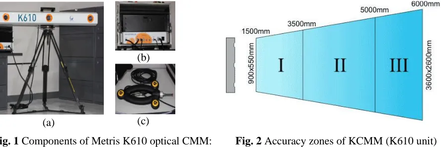
Dimensional inspection of large-sized objects are extensively involved in multiple stages in automotive industries, from design and prototyping up to in-line inspection supporting final assembly (Paul G Maropoulos et al. 2008, Jafar Jamshidi et al. 2010, Fiorenzo Franceschini et al. 2014). Traditional Cartesian CMM (e.g. Gantry and Horizontal-arm CMMs) is one of the best metrology solutions to large volume dimensional metrology applications (GN Peggs et al. 2009), provided that they incorporate high accuracy and reliability of the measurement result (W. T. Estler et al. 2002). However, in some applications where the measurand dimensions are larger than defined working volume of the system. Or in cases where the measurand is difficult to move in the measurement frame, the objects must be measured in situ. For applications in such cases portable measuring systems are more appropriate. K-Series Optical CMM (KCMM) is a portable CMM that faces no mechanical constraints capable of fitting an entire vehicle in its measuring volume (about 17 m3 _{for K610 camera system, see Fig. 1). A tactile probe is used to locate a}

2

NV 2016) volumetric accuracy is up to 100 µm within 6 meters depth of view, and single point accuracy is up to 67 µm. The indicated measurement uncertainty is expressed as the expanded uncertainty with a coverage factor of 2, according to the ISO 10360-2, VDI 2617 and ANSI / ASME B89.1.12M standards for acceptance of CMMs (International Organization for Standardization (ISO) 1993). It is stated (Nikon Metrology NV 2016) as well that the uncertainty over the whole FOV (field of view) is divided into three accuracy zones dependent on the depth of field (Fig. 2).

(a)

(b)

(c)

Fig. 1 Components of Metris K610 optical CMM: (a) camera array; (b) controller; (c) tactile probe

Fig. 2 Accuracy zones of KCMM (K610 unit)

The length inspection by KCMM is evaluated by measuring two endpoints that define the length. Given the 3D coordinates of two endpoints, the distance between these 2 points is calculated by Eq. 1. In practical use of KCMM, positioning the KCMM relative to the measurand is a non-trivial job, in order to obtain a measuring layout with lowest uncertainty. For example, to measure the same distance between two points, the result measured in zone I is more accurate than that in zone III (Table 1). However, if the distance to be measured is longer than the diagonal of each zone, the distance inevitably needs to be measured in more than one accuracy zone. For length inspection in this scenario two measurement strategies exist (J. L. Crowley and Y. Demazeau 1993, A. Y. K. Ho and T. C. Pong 1996, R. Labayrade et al. 2005, A Weckenmann et al. 2009, Maurizio Galetto et al. 2015, Fiorenzo Franceschini et al. 2016) (Fig. 3): (I) the first strategy is to position one endpoint in zone I (i.e. more accurate zone) and the other one in zone II or III (i.e. less accurate zones).

Table 1. Accuracy zones of K610 CMM

Accuracy

Zone Volumetric Accuracy Single Point Accuracy

I 90µm + 10 µm/m 60µm + 7 µm/m

II 90µm + 25 µm/m 60µm + 17 µm/m

III 190µm + 25 µm/m 130µm + 17 µm/m

3

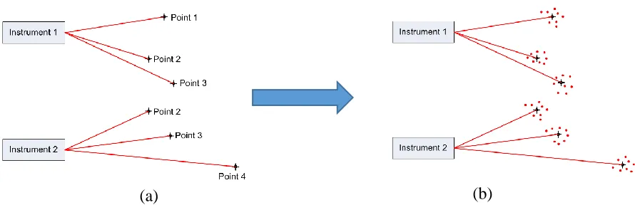
compared with the closer endpoint; (II) the second strategy is to measure one endpoint in zone I, and move the KCMM to the opposite end of the inspected length, and then measure that endpoint in zone I again. This method requires an additional alignment process for the two instrument positions used, in order to express two measurements in a common reference system. The uncertainty of length measured by the second strategy is subject to the added uncertainty introduced in alignment between two local coordinate systems of KCMM (J. E. Muelaner et al. 2010). The question this paper addresses is that, given the separated accuracy zones, what measurement strategy provides higher quality measurement results for length inspection (Fig. 3).

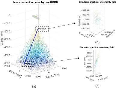
Fig. 3 Illustration of two measurement strategies of length inspection (LAB) on a generic car using K610

camera system (KCMM): in strategy (I), length between point A and point B is measured using one KCMM; in strategy (II), the length is measured from two positions of KCMM, provided overlapping area between both FOVs.

4

2. Two methods to determine the uncertainty of length measured

Length inspection using K-Series Optical CMM is carried out by measuring 3D coordinates of two endpoints (point A and point B in Fig. 3). The distance between point A and point B represents the value of length to be measured.

𝐿𝐴,𝐵 = ‖𝑃𝐴, 𝑃𝐵‖ = √(𝑋𝐴− 𝑋𝐵)2+ (𝑌𝐴− 𝑌𝐵)2+ (𝑍𝐴− 𝑍𝐵)2 (1)

The uncertainty of the measured length can be derived from the uncertainty of coordinate measurements of both endpoints, based on these assumptions: (i) the Cartesian coordinates measured at a single point follow a multivariate normal distribution, i.e. 𝑷_𝒊(𝑋_𝑃𝑖, 𝑌_𝑃𝑖, 𝑍_𝑃𝑖)~𝑁(𝝁_𝑷𝒊, ∑_𝑷𝒊) , where 𝝁_𝑷𝒊 and ∑_𝑷𝒊 are mean vector and covariance matrix, which can be estimated by the sample mean vector and sample covariance matrix respectively; (ii) Cartesian coordinates of two endpoints (i.e. 𝑷_𝒊(𝑋_𝑃𝑖, 𝑌_𝑃𝑖, 𝑍_𝑃𝑖), 𝑖 = 𝐴, 𝐵) are independently distributed random variables; (iii) all the correction and systematic compensation have been done, so only the random variability of coordinates measurement is considered here.

Two methods that propagate the uncertainties of the coordinates measurement into length measurement result are adopted in this paper—the Taylor Series Method (TSM) and the Monte Carlo Method (MCM) (Joseph M Calkins and Robert J Salerno 2000, IEC BIPM et al. 2008a, IEC BIPM et al. 2008b).

2.1 Taylor Series Method (TSM)

TSM is an analytical approach to propagate uncertainty and error, which is based on two main assumptions (H.W. Coleman and W.G. Steele 2009):

 The adequacy of the formula by which the derived variable is expressed as a function of measured variables;

 The distribution of derived variable is known, e.g., Gaussian or Student’s t-distribution, in order to obtain the value of coverage factor k.

The distance between two endpoints is a derived variable by combining all the measured values of different variables on right hand side in Eq. 1, the combined standard uncertainty of length variable (𝑢𝐿𝐴,𝐵) is thus derived by a first order Taylor Series Expansion formula (H.W. Coleman

and W.G. Steele 2009):

𝑢𝐿𝐴,𝐵 = √(∇𝐿𝐴) 𝑇_Σ

𝐴(∇𝐿𝐴) + (∇𝐿𝐵)𝑇Σ𝐵(∇𝐿𝐵) (2)

Where (∇𝐿𝑖)𝑇 ≡ ( 𝜕𝐿 𝜕𝑋𝑖,

𝜕𝐿 𝜕𝑌𝑖,

𝜕𝐿 𝜕𝑍𝑖)

𝑇_{, 𝑖 = 𝐴, 𝐵 is the gradient of L with respect to}

variables (𝑋𝑖, 𝑌𝑖, 𝑍𝑖)𝑇 , and Σ𝑖 ≡ [

𝜎_𝑋2_𝑖 𝜎_{𝑋𝑖𝑌𝑖} 𝜎_{𝑋𝑖𝑍𝑖} 𝜎𝑌𝑖𝑋𝑖 𝜎𝑌𝑖

2 _𝜎 𝑌𝑖𝑍𝑖 𝜎_{𝑍𝑖𝑋𝑖} 𝜎_{𝑍𝑖𝑌𝑖} 𝜎_𝑍2_𝑖

] , 𝑖 = 𝐴, 𝐵 is the covariance matrix

of (𝑋𝑖, 𝑌𝑖, 𝑍𝑖)𝑇. In practice, ∇𝐿𝑖 and Σ𝑖 are evaluated by the sample mean and sample covariance

5 2.2 Monte Carlo Method (MCM)

Rather than analytical method such as TSM, numerical methods such as Monte Carlo simulation, provide an alternative approach to uncertainty evaluation using sampling techniques. Such techniques are useful for validating the results obtained by TSM, as well as in the cases where the assumption made by TSM do not hold. To apply MCM, a distribution is assumed to each variable on the right hand side of Eq. 1, which has been stated above, and a number of iterations is run until a converged value for standard deviation of the derived variable 𝑠𝑀𝐶𝑀is achieved,

then 𝑢_{𝐿𝐴,𝐵} = 𝑠_𝑀𝐶𝑀, meanwhile, the distribution of the derived variable is obtained as well. It needs to be mentioned that 𝑠_𝑀𝐶𝑀 is the estimate of the combined standard uncertainty of 𝑢_{𝐿𝐴,𝐵} . We do not need to have a perfectly converged value of 𝑠𝑀𝐶𝑀 to have a reasonable estimate of

𝑢𝐿𝐴,𝐵 . Once the 𝑠𝑀𝐶𝑀 values are converged to within 1–5%, then the value of 𝑠𝑀𝐶𝑀 is a good

approximation of the combined standard uncertainty of the result. The level of convergence is a matter of judgment based on the cost of the sampling process and the application for 𝑢_{𝐿𝐴,𝐵} . Once a converged value of 𝑢𝐿𝐴,𝐵 is determined and assuming that the central limit theorem applies, the

expanded uncertainty for the result at a 95% level of confidence is U = 2 𝑢_{𝐿𝐴,𝐵}(H. W. Coleman and W. G. Steele) .

3. Metrology model of K610 camera system

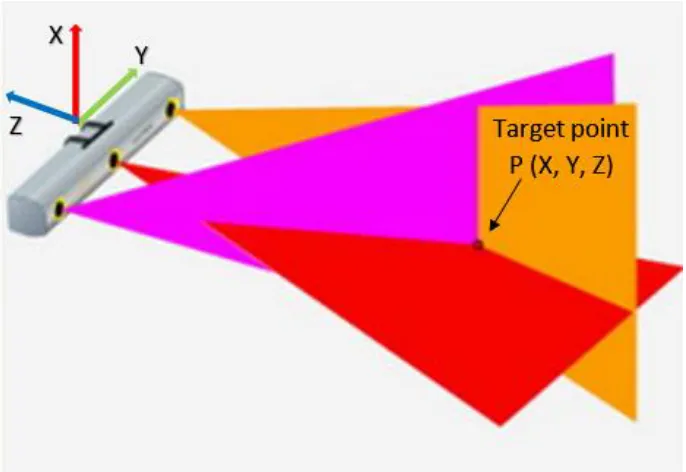
A KCMM system can be used for handheld and robotized 3D inspection, motion analysis and robot metrology. Regardless of the application, the measurement principle is the same. Three linear CCD (Charge-Coupled Device) cameras are placed in a linear-based layout, each of them measures one angle from optical center to the target point, three angles are integrated to localize the target point, based on triangulation principle (Fig. 4).

6 3.1 Technical parameters of K610 CMM

Fig. 5 A generic model of 3-cameras system (in 2D).

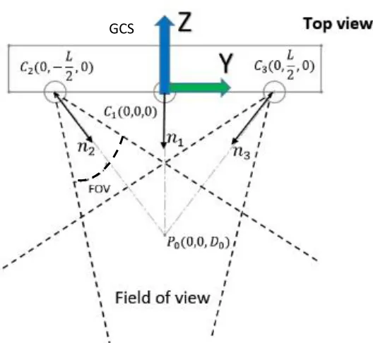
A generic model of the 3-cameras system (M. Galetto and L. Mastrogiacomo 2013, J. Caja et al. 2015) is modeled in 2D as illustrated in Fig. 5. A virtual line is supposed to pass through the optical observation centers of the 3 cameras, with the middle camera numbered as C1, the left one numbered as C2 and the right one numbered as C3, respectively. A global coordinate system is established with the y-axis passing from camera C2 to camera C3, and the z-axis is perpendicular to y-axis, pointing backwards of the cameras’s FOV. The position of 3 cameras with respect to global coordinate system (GCS) is shown in Fig. 5, assuming the distance between two outer cameras is L, and the two outer cameras are placed symmetrically about the center camera. The local coordinate system (LCS) of each camera is shown in Fig. 6, where the sensor is aligned with y-axis and the target point is mapped by sensors of each camera onto the local y-z plane. The output of the sensor is one angle formed by the projection line that passes from the observation center to the target point, and the normal vector. The cameras are oriented towards a point 𝑃₀(0,0, 𝐷₀) in front of the center camera. With this layout, the X-coordinate of target point is determined by the center camera C1, while the Y and Z-coordinates are determined by the outer cameras C2 and C3 together (A. Lamallem et al. 2009).

3.2 Localization scheme of 3D points

The sensor readings from 3 linear CCD cameras are 3 angles ( 𝜃₁, 𝜃₂ , 𝜃₃ ) from each camera respectively. The Y and Z coordinates defined by 𝜃2 and 𝜃3 together, while X coordinate is

defined only by 𝜃1alone. The relation between output (X, Y and Z coordinates) and the sensor

readings ( 𝜃₁, 𝜃₂ , 𝜃₃ ) is shown in Eq. 3:

7

𝑍 = −𝐿 ( 1

tan(𝜙 − 𝜃₂)+

1

tan(𝜙 + 𝜃₃))

(3)

𝑌 = −𝑍

tan (𝜙 − 𝜃₂)− 𝐿 2

𝑋 = −𝑍 ∗ tan(𝜃1)

where 𝜙 = atan ( 𝐷

𝐿 2⁄ ) is a constant angle determined by D and L. Given a generic model of the

camera system and pressumed uncertainty value (normal distribution, standard deviation = 1/3600 degree, i.e. 1 second) of angular sensor (Rene Wackrow et al. 2007, Jody E Muelaner et al. 2009), a simulation as illustrated in Fig. 7 was run by building the camera model with following parameters (Table 2):

Table 2. Camera model parameters

Parameter name: Parameter value:

L 1000 mm

D0 6000 mm

FOV ± 16.70 degrees

sigma 1 arc second

Fig. 6 a generic model of a linear CCD sensor

The simulation comprised of a population of 100,000 points uniformly distributed in a space with 6 m × 6 m × 6 m in three dimensions, and approximately 10 percent of the points (distributed in a simulated working volume of 17 m³) are covered by 3 cameras all together, these 10 percent points formed a pyramidal shape shown in Fig. 7.

Fig. 7 Pyramidal FOV of KCMM

8

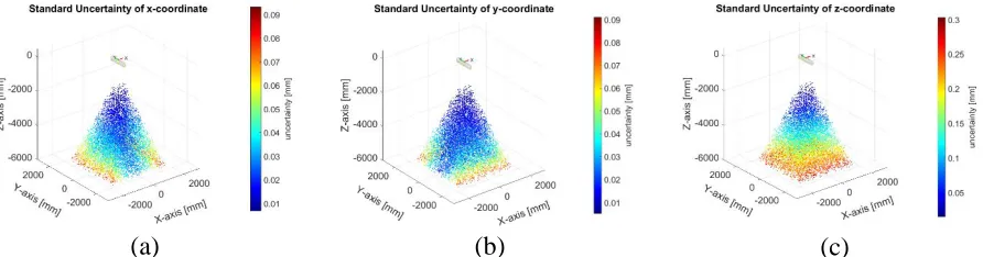
3000 repeated coordinates measurements of each point were run and the standard uncertainty of each X, Y and Z-coordinate was estimated based on the simulated 3D coordinates, the uncertainty map of X, Y and Z-coordinate is shown in Fig. 8-a, 8-b and 8-c respectively.

(a) (b) (c)

Fig. 8 Standard deviation (unit in color bar: mm) of (a) x-coordinate (b) y-coordinate (c) z-coordinate, respectively (unit: mm), in FOV, from simulation.

The generic camera model is a first approximation of the KCMM system, this model is quite useful to simulate the uncertainty field of a single point measurement, and the result is validated by the experiment data, to the extent that the uncertainty of a single point measurement in the measuring volume is related to the z-coordinate of that point. This model is subject to a bias from the true KCMM model. For commercial reasons the true values of camera parameters are not released by the manufacturer. A more realistic model can be defined if such parameters could be given by the instrument manufacturer. Even at its current state the virtual model is useful in planning a measuring scheme. Given the distribution of uncertainty map, an optimal layout of experiment can be planned in advance of digitization process (Fiorenzo Franceschini et al. 2015).

4. Proposed strategies for length inspection, simulation and physical experiment

4.1 Length inspection by first strategy

Length inspection using one single position for KCMM system is carried out by measuring the Cartesian coordinates of two endpoints of an artefact (e.g. a calibrated long bar). The length value is the distance between the two endpoints, and the uncertainty of measured length is determined by the uncertainty of measurements of Cartesian coordinates (see Eq. 2). A repeated simulation of Cartesian coordinates’ measurements is carried out, in the following steps:

Step 1: A long bar (with pre-defined nominal length, e.g. 5000 mm) is randomly placed in the FOV, with one endpoint placed in accuracy Zone-I (see Fig. 2) while the other placed in accuracy Zone-II or Zone-III, according to the nominal length;

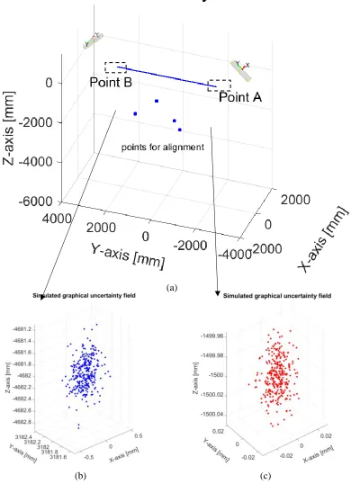
Step 2: 300 repeated measurements are simulated for both two points, in order to demonstrate the uncertainty field of both. The length measurement result is determined by Eq. 1 and the uncertainty of that is calculated by i) TSM and ii) MCM; a graphical uncertainty field is illustrated in Fig. 9, (b) for point A and (c) for point B;

9

Step 4: The nominal length of bar is changed and steps 1 to 3 are repeated. The nominal length ranged from 5000 mm down to 2000 mm.

(a)

(b)

(c)

Fig. 9 Demonstration of simulation scheme using one KCMM (coordinate system unit: mm): (a) the coverage of FOV of one KCMM; (b) graphical uncertainty field of point A (300 repeated simulations); (c) graphical uncertainty field of point B (300 repeated simulations).

4.2 Length inspection using two KCMM cooperatively

In the cases where the variability of coordinates of one endpoint dominates that of the other, it is reasonable to measure one endpoint in the more accurate zone of the instrument, while doing the same to the other endpoint. Afterwards, the measured 3D coordinates must be expressed in the same coordinate reference system. Therefore, overlapping area between two positions of the instrument must be inspected, in order to align one coordinate system to the other. The steps of simulation are listed as follows:

Step 1: A long bar with pre-defined nominal length (e.g. 5000 mm) is placed at a fixed position, where the midpoint is located at origin of the coordinate system, and the direction of the bar stayed parallel to the y-axis;

10

Step 3: 4 randomly selected points (the reason for selecting 4 points is explained in section 4.3) in the overlapping area of both KCMMs’ FOV are measured. Then the linear transformation from the second KCMM to the first KCMM are calculated through Procrustes algorithm;

Step 4: the uncertainty of length of the bar is calculated by i) TSM and ii) MCM, based on the uncertainty of coordinates measurement of point A by the first KCMM and point B transformed to the first KCMM’s coordinate reference system;

Step 5: change the relative positions and orientations between two KCMMs, repeat step 1 to step 4;

Step 6: The nominal length of bar is changed and steps 1 to 3 are repeated. The nominal length used range from 5,000 mm down to 2,000 mm.

The simulation scheme using two KCMMs is illustrated in Fig. 10.

4.3 Alignment scheme for the second strategy

11

(a)

(b) (c)

12

(a) (b)

Fig. 11 (a) Example of 2-dimensional measurement of 4 points using 2 instruments; (b) Measured points with simulated “uncertainty fields” around them. (adapted from (J. E. Muelaner et al. 2010) ,

with permission)

Fig. 12 Instrument position 2 located relative to instrument position 1 by best fitting the common points. (adapted from (J. E. Muelaner et al. 2010), with permission)

13

Fig. 13 Standard deviation of length (combined measurement by TSM method) versus nominal length (with different number of points in the overlapped metrology area, from 4 points to 10 points).

Fig. 13 illustrates no significant improvement (i.e. lower uncertainty in length measurement) when the number of overlapping points are increased from 4 to 10, in order to run best-fitting process between two positions of instrument. Therefore, to reduce the measurement cost and computational load, 4 points in the overlapping area are used to run best-fitting algorithm.

4.4 Case study

The experiment was conducted in the PVCIT Laboratory, the measured artefact was the BIW of a sports utility vehicle (SUV), which was fixed on a stable steel fixture. The approach employed in this work involves the use of kinematic nests, shown in Fig. 14, to allow the repeatable positioning of the probe involved in KCMM system.

(a) (b)

14

The layout of experimental scheme is shown in Fig. 15, in which 7 kinematic nests are divided into 2 groups: (i) point A and point B are taken as the endpoints of the length to be measured a; (ii) point 1 to point 5 are regarded as overlapping points measured to align two local coordinate systems of KCMM.

Fig. 15 Layout of the experimental scheme of on BIW of a SUV car.

5. Result discussion

The results of simulation and experiment are discussed in the following sections.

5.1Simulation result

A series of 7 length values (from 5000 mm to 2000 mm, with 500 mm decrements) have been used as nominal values to run length inspection simulation. In simulations by the first strategy, 1000 different positions and directions of each measured length are simulated (see Fig. 16-a). A group of 300 repeated measurements is carried out at each position and direction. In simulations by the second strategy, 7 different relative positions and orientations of two KCMMs are adopted for each measured length (see Fig. 16-b). Furthermore, at each position and orientation of KCMMs, 100 different sets of overlapping points are used (i.e. 4 randomly selected points in the overlapping area, measured in order to align between the two KCMMs’ coordinate reference systems). The purpose here was to investigate the effectiveness of alignment resulting from points’ selection in the overlapping area.

Point A

Point 3

Point 2

Point 1 Point 4

Point B

15

(a) (b)

Fig. 16 Demonstration of simulation scheme: (a) simulation using one KCMM, 1000 different directions of the measured bar (bar in blue color with nominal length 5000 mm) are plotted, one endpoint of the bar is placed at the plane z=-1500, while the other endpoint is placed randomly; (b) simulation using two KCMMs, four different tilt angles of KCMMs are plotted (tilt angle changes from 0° to 90°).

Simulated results from single KCMM case are shown in Fig. 17, in which the two methods (‘TSM’ and ‘MCS’ methods) of uncertainty propagation are compared. This shows no significant difference between the two methods. This verifies the effectiveness of the proposed method described by Eq. 2. The combined uncertainty of length measurement (||AB||) is plotted in Fig. 17 for different values of nominal length. Each boxplot represents the dispersion of uncertainty of length among 1000 different positions and directions of the measured artifact. It is shown that the median value of uncertainty of length increases with the nominal length, so does the dispersion of uncertainty. This is because the uncertainty of endpoint at further distance from the KCMM’s cameras dominates that of the other endpoint. Thus the UL increases as the distance ||AB|| increases. Specifically, considering the sixth boxplot on the left hand side as an example, this represents the dispersion of UL about the artifact whose nominal length 4,500 mm, and the maximum and minimum uncertainty are approximately 0.28 mm and 0.19 mm, respectively.

Simulated results from two positions of KCMM are shown in Fig. 18 and Fig. 19. In Fig. 18, the dispersion of UL by two KCMMs is plotted against the relative positions and orientations of the two KCMMs with the artifact. Each boxplot represents the dispersion of uncertainty among 100 different random selection of overlapping points to do alignment between two local coordinate systems. It can be seen that, the median value of uncertainty decreases with the tilt angle of the KCMM with respect to the artifact, so does the dispersion of uncertainty. It can be explained that, as the tilt angles of the two KCMMs increases, more overlapping area is covered by both KCMMs, thus the effectiveness of alignment increases, resulting in smaller uncertainty in alignment (J. E. Muelaner et al. 2010). Besides, it can be concluded that there is no significant difference between uncertainty dispersion when the tilt angle reaches 60° and higher.

Fig. 19, shows the dispersion of UL against different nominal lengths, given the same tilt angle (60°) of two KCMMs. Each boxplot represents the dispersion of uncertainty among 100 different random selection of overlapping points to run alignment algorithm. It is shown from Fig. 19 that, the median value of UL increases as the nominal length increases, this can be explained by the

0°

90°

90°

16

fact that, as the nominal length increases, the overlapping area between two KCMMs is farther from both KCMMs, which results in a higher uncertainty in measuring those overlapping points from both KCMMs, and in a higher uncertainty of coordinates of the transformed endpoint as a result.

(a) (b)

Fig. 17 Simulated results by single KCMM.

17

Fig. 19 Uncertainty of length simulated using two positions of KCMM (with 60° tilt angle), against different nominal lengths.

(a) (b)

Fig. 20 Comparison between two measuring strategies: (a) nominal length of 2000 mm; (b) nominal length of 5000 mm.

18

second case where nominal length to be measured is 5,000 mm, both in terms of median value and the lower limit (i.e. the best performance can be achieved) of the uncertainty.

As a summary, strategy-I achieves better performance than strategy-II in length measurement, in the sense that the dispersion of uncertainty is lower in any cases. However, when the nominal length to be measured reaches the capability threshold of single KCMM (e.g. 5,000 mm), strategy-II is more appropriate, in order to achieve lower UL. It has to be mentioned that, to achieve the best performance from strategy-II, the overlapping points for alignment need to be optimally selected, e.g. a proper number of overlapping points are used and they are opportunely positioned between the common FOV of two KCMMs.

5.2Result from experiment data

The experimental scheme for length inspection is illustrated in Fig. 21. All the 7 points are measured repeatedly (15 replications each point) from two positions of KCMM (namely KCMM1 and KCMM2), and 4 different scenarios are considered in the experiment: i) ||AB|| (i.e. the length between point A and point B) is measured by KCMM1 alone; ii) ||AB|| is measured by KCMM2 alone; iii) point A is measured by KCMM1, while point B is measured by KCMM2 and transformed into KCMM1’s coordinate system; iv) point B is measured by KCMM2, while point A is measured by KCMM1 and transformed into KCMM2’s coordinate system. The scenarios i) and ii) represent the cases that KCMM measure the length alone, while scenarios iii) and iv) represent the cases that two KCMMs do measurement cooperatively. The measurement result is listed in Table 3.

Table 3 Coordinates measurements by strategy-II (unit: mm).

case (i) case (ii) case (iii) case (iv)

Length

||AB||

best

estimation 1704.518 1704.481 1704.462 1704.491

combined

uncertainty 0.034 0.016 0.045 0.048

19

Fig. 21 Experimental scheme demonstration.

6 Conclusion

This paper focuses on the uncertainty characteristics of a class of camera-based measuring systems (i.e. K-series CMM from Nikon Metrology) and discusses a metrology model of KCMM by an experimental method. Furthermore, the paper describes two methods to propagate the uncertainty of length inspection (Monte-Carlo Simulation and Taylor Series Method) based on the uncertainty propagation of coordinates measurement. A simulation scheme is proposed to compare two different strategies of conducting point to point (length) inspection. The simulated result is justified by an experiment that was carried out on an SUV body.

Camera-based measuring systems such as K-series CMM system measures a spatial point based on triangulation principles. This results in a depth-dependent uncertainty field of KCMM. As a consequence, two strategies of length inspection come into being, for measuring with portable instruments. Specifically, the first strategy is to cover the measured length in the FOV of a single KCMM, while the second strategy is to split the measured length in different FOVs of two KCMMs, and the length is measured by merging the results by two KCMMs.

Z-axis [m

m

20

According to simulated and experimental results, the first strategy achieves smaller UL compared to the second one, in a wide range of scenarios. However, the second strategy can achieve better performance in the best cases, by optimally selecting those points for registering two sets of local measurements.

Future research could focus on the potential of the measuring strategy that involves two or more measuring systems cooperatively, as is discussed in this paper. Great attention and dedicated methods may be required to coordinate and cooperate multiple systems together, in order to achieve a better metrological performance.

References

International Organization for Standardization (ISO) (1993). Guide to the Expression of Uncertainty in Measurement,. ISO, Geneva.

IEC BIPM, ILAC IFCC, IUPAP IUPAC and OIML ISO (2008a). Evaluation of measurement data— guide for the expression of uncertainty in measurement. JCGM 100: 2008, ed.

IEC BIPM, ILAC IFCC, IUPAP IUPAC and OIML ISO (2008b). "The international vocabulary of metrology—basic and general concepts and associated terms (VIM), 3rd edn. JCGM 200: 2012." JCGM (Joint Committee for Guides in Metrology).

J. Caja, E. Gómez and P. Maresca (2015). "Optical measuring equipments. Part I: Calibration model and uncertainty estimation." Precision Engineering 40: 298-304.

Joseph M Calkins and Robert J Salerno (2000). A practical method for evaluating measurement system uncertainty. Proceedings of the 2000 Boeing Large Metrology Conference, Long Beach, CA, USA. H.W. Coleman and W.G. Steele (2009). Experimentation, Validation, and Uncertainty Analysis for Engineers, Wiley.

J. L. Crowley and Y. Demazeau (1993). "Principles and techniques for sensor data fusion." Signal Processing 32(1-2): 5-27.

W. T. Estler, K. L. Edmundson, G. N. Peggs and D. H. Parker (2002). "Large-scale metrology - An update." CIRP Annals - Manufacturing Technology 51(2): 587-609.

Fiorenzo Franceschini, Maurizio Galetto and Gianfranco Genta (2015). "Multivariate control charts for monitoring internal camera parameters in digital photogrammetry for LSDM (Large-Scale Dimensional Metrology) applications." Precision Engineering 42: 133-142.

21

Fiorenzo Franceschini, Maurizio Galetto, Domenico Maisano and Luca Mastrogiacomo (2016). "Combining multiple Large Volume Metrology systems: Competitive versus cooperative data fusion." Precision Engineering 43: 514-524.

M. Galetto and L. Mastrogiacomo (2013). "Corrective algorithms for measurement improvement in MScMS-II (mobile spatial coordinate measurement system)." Precision Engineering 37(1): 228-234.

Maurizio Galetto, Luca Mastrogiacomo, Domenico Maisano and Fiorenzo Franceschini (2015). "Cooperative fusion of distributed multi-sensor LVM (Large Volume Metrology) systems." To appear on CIRP Annals Manufacturing Technology DOI:10.1016/j.cirp.2015.04.003.

John C Gower and Garmt B Dijksterhuis (2004). Procrustes problems. Oxford, UK, Oxford University Press Oxford.

A. Y. K. Ho and T. C. Pong (1996). "Cooperative fusion of stereo and motion." Pattern Recognition 29(1): 121-130.

Jafar Jamshidi, A Kayani, Pejman Iravani, Paul G Maropoulos and MD Summers (2010). "Manufacturing and assembly automation by integrated metrology systems for aircraft wing fabrication." Proceedings of the Institution of Mechanical Engineers, Part B: Journal of Engineering Manufacture 224(1): 25-36.

R. Labayrade, C. Royere, D. Gruyer and D. Aubert (2005). "Cooperative fusion for multi-obstacles detection with use of stereovision and laser scanner." Autonomous Robots 19(2): 117-140.

A. Lamallem, L. Valet and D. Coquin (2009). Local versus global evaluation of a cooperative fusion system for 3D image interpretation. ISOT 2009 - International Symposium on Optomechatronic Technologies, Istanbul, IEEE.

Paul G Maropoulos, Y Guo, Jafar Jamshidi and Bin Cai (2008). "Large volume metrology process models: A framework for integrating measurement with assembly planning." CIRP Annals-Manufacturing Technology 57(1): 477-480.

Edward M Mikhail, James S Bethel and J Chris McGlone (2001). Introduction to modern photogrammetry, John Wiley & Sons Inc.

J. E. Muelaner, Z. Wang, O. Martin, J. Jamshidi and P. G. Maropoulos (2010). "Estimation of uncertainty in three-dimensional coordinate measurement by comparison with calibrated points." Measurement Science and Technology 21(2).

22

Nikon Metrology NV (2016). "

http://www.nikonmetrology.com/en_EU/Products/Portable-Measuring/Optical-CMM/K-Series-Optical-CMM/(specifications)." Retrieved 16 March, 2016.

GN Peggs, Paul G Maropoulos, EB Hughes, AB Forbes, S Robson, M Ziebart and B Muralikrishnan (2009). "Recent developments in large-scale dimensional metrology." Proceedings of the Institution of Mechanical Engineers, Part B: Journal of Engineering Manufacture 223(6): 571-595.

Heinrich Schwenke, Ulrich Neuschaefer-Rube, Tilo Pfeifer and Horst Kunzmann (2002). "Optical methods for dimensional metrology in production engineering." CIRP Annals-Manufacturing Technology 51(2): 685-699.

George AF Seber (2009). Multivariate observations, John Wiley & Sons.

Rene Wackrow, Jim H Chandler and Paul Bryan (2007). "Geometric consistency and stability of consumer‐grade digital cameras for accurate spatial measurement." The Photogrammetric Record 22(118): 121-134.