Bayesian spatial monotonic multiple regression

Advance Access publication on 31 July 2016

Printed in Great Britain

Bayesian spatial monotonic multiple regression

BYC. ROHRBECK, D. A. COSTAIN

Department of Mathematics and Statistics, Lancaster University, Lancaster LA1 4YF, U.K. [email protected] [email protected]

ANDA. FRIGESSI 5

Department of Biostatistics, University of Oslo, PB 1122 Blindern, 0317 Oslo, Norway. [email protected]

SUMMARY

We consider monotonic, multiple regression for contiguous regions. The regression functions vary regionally and may exhibit spatial structure. We develop Bayesian nonparametric methodol- 10

ogy that permits estimation of both continuous and discontinuous functional shapes using marked point process and reversible jump Markov chain Monte Carlo techniques. Spatial dependence is incorporated by a flexible prior distribution which is tuned using cross-validation and Bayesian optimization. We derive the mean and variance of the prior induced by the marked point process approach. Asymptotic results show consistency of the estimated functions. Posterior realizations 15

enable variable selection, the detection of discontinuities and prediction. In simulations and in an application to a Norwegian insurance data set, our methodology shows better performance than existing approaches.

Some key words: Cross-validation; Isotonic regression; Marked point process; Optimization; Reversible jump Markov

chain Monte Carlo algorithm; Spatial dependence. 20

1. INTRODUCTION

Geospatial data are considered in forestry (Penttinen et al., 1992), epidemiology (Waller & Gotway, 2004) and other domains. Due to practicality or confidentiality concerns, locally ag-gregated data are common and are typically available on an irregular lattice. Statistical methods for such data aim to explore the association between a response and explanatory variables while 25

accounting for spatial dependence in the model parameters. To introduce such dependence, a neighbourhood structure, often based upon the arrangement of the areal units on a map, is typi-cally defined via an adjacency matrix.

Most modelling frameworks assume a common effect of the explanatory variables for all re-gions (Waller & Gotway, 2004; Wakefield, 2007). Spatial variation is then typically accommo- 30

dated via a spatially structured random effect on the intercept. Some applications, however, need to allow for a spatially-varying regression function (Bell et al., 2004; Zhang & Shi, 2004; Cahill & Mulligan, 2007). Statistical methods for such scenarios are available for generalized linear (Fotheringham et al., 2003; Assunc¸˜ao, 2003; Scheel et al., 2013) and additive models (Cong-don, 2006). However, these approaches are limited, as continuity of the regression function is 35

assumed: abrupt changes in the regression surface are not captured unless they are explicitly included in the model. Neglecting such effects may result in a bias due to oversmoothing; see Bowman & Azzalini (1997) p.26.

C

Since continuity may be inappropriate, we replace it by monotonicity (Royston, 2000; Farah et al., 2013; Wilson et al., 2014). Whilst continuity cannot, in general, be verified, tests of

mono-40

tonicity are available (Bowman et al., 1998; Ghosal et al., 2000; Scott et al., 2015). Based upon a number of observations for each region, we develop Bayesian nonparametric methodology which estimates the regional regression functions whilst exploiting any neighbourhood structure.

The estimation of a single monotonic function is usually called isotonic regression. Early publications discuss inference under monotonicity constraints (Ayer et al., 1955; Brunk, 1955;

45

Barlow & Brunk, 1972) and solution algorithms are available (Brunk et al., 1957; Luss et al., 2012). Isotonic regression is further considered for additive (Bacchetti, 1989; Tutz & Leitenstor-fer, 2007) and high-dimensional models (Fang & Meinshausen, 2012; Bergersen et al., 2014), in functional data analysis (Ramsay, 1998; Ramsay & Silverman, 2005) and Bayesian nonparamet-ric modelling (Gelfand & Kuo, 1991; Shively et al., 2009; Saarela & Arjas, 2011; Lin & Dunson,

50

2014). In order to learn about potentially spatially structured monotonic regression functions, a dependence model for functions, possibly with discontinuities, is required.

Our approach represents each monotonic regional function by a set of marked point processes. Potential spatial structure is modelled via a joint prior distribution, which is based upon a flexi-ble discrepancy measure. The prior allows the functional dependence to be constant, increasing

55

or decreasing with increasing function values. The Bayesian framework induces a consistent posterior (Barron et al., 1999; Walker & Hjort, 2001), and permits both smooth contours and discontinuities. To tune the prior, we combine cross-validation and Bayesian optimization. Real-izations of the posterior are obtained by a reversible jump Markov chain Monte Carlo algorithm (Green, 1995) and enable variable selection, prediction and the detection of discontinuities.

60

2. MODELLING ANDINFERENCE 2·1. Likelihood and notation

ConsiderKcontiguous regions whose neighbourhood structure is given by an adjacency ma-trix or a lattice graph. Letyk∈Randxk∈Rm denote the response and explanatory variables,

respectively, for regionk(k= 1, . . . , K). The likelihood is

65

f{yk |λk(xk), θk}, (1)

where λk:Rm→[δmin, δmax] is the monotonic regression function for region k, for which λk(xk)is assumed to lie within the predefined interval[δmin, δmax]. Monotonicity is defined in terms of the partial Euclidean ordering: ifu≤vcomponent-wise,λk(u)≤λk(v),u, v∈Rm.

The vectorθkdenotes additional, potentially spatially varying, model parameters which are a pri-ori independent ofλ1, . . . , λK.

70

In what follows, we perform inference onλ1throughλKwhile accounting for potential spatial structure in these functions. Each λk (k= 1, . . . , K) is estimated over a closed setX ⊂Rm.

In applications, X and [δmin, δmax]may be defined in terms of the explanatory variables and responses, respectively. For instance, ifλk(xk)in (1) is the mean response,δminmay be set to the minimum observed response across theKregions. In§2·2 to§2·4 we complete the Bayesian

75

framework by defining a joint prior on λ1, . . . , λK while §2·5 and §2·6 detail the estimation procedure.

2·2. A spatial dependence model for the monotonic functions

We wish to impose spatial structure on λ1, . . . , λK and hence define a joint prior density that favours these functions to be similar. We set δmin= 0 and writeλk(x)instead ofλk(x)−

80

0.0 0.5 1.0 1.5 2.0

0

1

2

3

4

γp

{

κ

,

ψ

}

κ

0 1 2 3 4

0

1

2

3

4

5

γp

{

κ

,

ψ

}

/

γp

{

0

,

1

}

κ

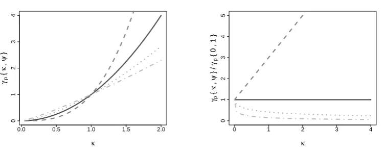
Fig. 1. Behaviour ofγp{κ, ψ}with respect toκforp= 1 ( ),p= 2( ),p= 0·5( ) andp= 0·2( ), subject toψ= 0(left) andψ=κ+ 1(right) being fixed.

First, we introduce a pairwise discrepancy measure forλkandλk0 (k, k0 = 1, . . . , K; k6=k0).

Such a measure should be minimal if and only ifλkandλk0 are equal, and should increase with

an increasing difference in these functions. A possible choice is the integrated squared distance

Z

X

{λk(x)−λk0(x)}2 dx. (2)

Sometimes, we may have prior knowledge that differences in the lower, or higher, function 85

values of λk and λk0 should be downweighted, or avoided. For example, increased

measure-ment error in higher values of the explanatory variables may be better handled through increased information borrowing. Thus, we replace{λk(x)−λk0(x)}2in (2) by

γp{λk(x), λk0(x)}= [ {λ_k(x)}p− {λ_k0(x)}p ] {λ_k(x)−λ_k0(x)}, p >0, (3)

for whichp= 1yields the integrated squared distance. See the 2017 Lancaster University PhD thesis by C. Rohrbeck for a more general formulation. Expression (3) can also be interpreted as 90

the squared distance with weight[{λk(x)}p− {λk0(x)}p]/{λ_k(x)−λ_k0(x)}.

Figure 1 illustrates the behaviour ofγp{λk(x), λk0(x)}at a fixed pointx∈_Rm for different

settings of p. For brevity, let κ=λk(x) andψ=λk0(x). The left panel shows that γ_p{κ, ψ}

increases with an increasing difference betweenκ andψ= 0 for all settings of p. Hence, γp satisfies the desired properties stated above. Furthermore in the right panel, the fixed difference 95

ψ=κ+ 1 is penalized more for higher κ if p >1, while being penalized less for p <1. A constant penalty is induced forp= 1. As such, the parameterpallows the penalty for differences betweenλkandλk0 to vary with the function values.

The dependence model for theK-setλ1, . . . , λK is then defined as a Gibbs measure (Georgii, 2011) with the discrepancy measure constructed in (2) and (3) as a pair-potential. Formally, 100

π(λ1, . . . , λK |ω)∝ Y

1≤k<k0_≤K

exp

−ω dk,k0

Z

X

γp{λk(x), λk0(x)} dx

, ω ≥0, (4)

where the product is over all pairs of regions. The constantdk,k0 ≥0describes our prior belief

concerning the degree of similarity ofλkandλk0. In spatial statistics, we often setd_k,k0 = 1if the

regionskandk0are adjacent anddk,k0 = 0otherwise. Such a choice reduces the computational

0.0 0.2 0.4 0.6 0.8 1.0

0.0

0.2

0.4

0.6

0.8

1.0

x1

x2

Fig. 2. Point locations to represent a step functionλ on X = [0,1]2 via a set of I= 3 marked point processes (∆1,∆2,∆3). The processes∆1( ),∆2( ) and∆3( )

are defined on the setsX1= [0,1]×0, X2= 0×[0,1]

andX3= (0,1]×(0,1], respectively.

to choice of p is explored in §3·3. Expression (4) can be extended to regionally varying X, permitting borrowing of information for extrapolation; see the Supplementary Material.

2·3. Marked point process prior

We specify an individual prior model forλk:X →[δmin, δmax] (k= 1, . . . , K) and drop the index k in the rest of this subsection for brevity. Prior distributions proposed in the literature

110

include an ordered Dirichlet process (Gelfand & Kuo, 1991) and a constrained spline (Shively et al., 2009). Our prior is similar to that of Saarela & Arjas (2011): λ is postulated to be a non-decreasing step function withλ(x)∈[δmin, δmax]; any monotonic, bounded function can be approximated to a desired accuracy by increasing the number of steps.

The location and height of the steps of λdefine a marked point process on X. Following

115

Saarela & Arjas (2011), we representλvia a set ofImarked point processes,∆ = (∆1, . . . ,∆I), where∆i(i= 1, . . . , I) is on a setXiwithSIi=1Xi =X. Here, we defineX1, . . . , XIbased on the non-empty subsets of{1, . . . , m}. For example, ifm= 2we chooseI = 3and have separate processes∆1and∆2for each of the two explanatory variables,x1andx2, respectively, and one process∆₃for both components,(x1, x2), jointly. Figure 2 provides an example forX = [0,1]2.

120

The benefits of this representation are discussed later in this subsection. We now formalize the representation ofλvia∆and denote

∆i ={(ξi,j, δi,j)∈Xi×[δmin, δmax] : j= 1, . . . , ni}, i= 1, . . . , I. (5)

Here, ξi,j and δi,j refer to a point location and associated mark, respectively, and ni is the number of points in ∆i. Monotonicity is imposed by constraining the marks: if ξi,j ξi0_,j0,

δi,j ≤δi0_,j0 (i, i0 = 1, . . . , I;j= 1, . . . , ni;j0 = 1, . . . , n_i0). The valueλ(x)is then defined as 125

the largest markδi,j such thatximposes a monotonicity constraint on the associated point loca-tionξi,j. Formally,

λ(x) = max

i,j {δi,j : ξi,j x}. (6)

val-ues ofx1, that is,λ(x) =λ{x+ (,0, . . . ,0)}(x∈X; >0). As we representλvia a marked 130

point process, the redundancy ofx1 implies that the point locations are in the set0×[0,1]m−1. For instance, ifm= 2, all points then lie on the linex1= 0in Fig. 2. As such, the processes∆1 and∆₃ contain no points. Consequently,ni (i= 1, . . . , I) provides an indicator of the redun-dancy of explanatory variables.

The association defined in (6) results in a mapping between the spaces of step functions and 135

marked point processes with monotonicity constraints. Thus, we can define a prior forλvia one for∆. A priori, the numberN =PI

i=1ni of steps representingλis geometrically distributed with probability 1/η (η >1) and N = 0 corresponds to λ=δmin being constant. This choice promotes model parsimony and favoursλto have few steps. GivenN, the vector(n1, . . . , nI) is uniformly distributed over the set of possibilities of allocatingN points to theI processes. 140

For ∆i (i= 1, . . . , I), the location ξi,j (j = 1, . . . , ni) is uniformly distributed on Xi. The marks{δi,j : j = 1, . . . , ni; i= 1, . . . , I}are uniformly distributed on[δmin, δmax], subject to the monotonicity constraints imposed by the locations in ∆₁, . . . ,∆I. Using this hierarchical structure, we obtain the prior density

φ(∆|η) =π({δi,j} | {ξi,j})    I Y i=1 ni Y j=1 π(ξi,j)

 



π(n1, . . . , nI |N)π(N |η) ; (7)

further details are provided in the Supplementary Material. 145

The densityφ(∆|η)induces a density on the space of step functions,φ˜(λ|η), which can be characterized as follows:

PROPOSITION1. LetX = [0,1], δmin= 0andδmax= 1. Then the distribution with density ˜

φ(λ|η)has

E{λ(x)|η}=x

∞ X n=1 ₁ η

1−1

η

n _n

n+ 1

=x

1− logη

η−1

, 150

var{λ(x)|η}=

∞ X n=1 ₁ η

1−1

η

n_nx(2−x+nx)

(n+ 1)(n+ 2)

−E{λ(x)|η}2.

Hence, the expectation is a linear function whose slope depends onη. See the Supplementary Material for the the proof of Proposition 1.

This Bayesian framework has one small limitation. If, for instance,X= [0,1],λ(0) =δmin al-most surely. To address this, we defineλ(x) =µ+ϕ(x), whereϕ:X→[δmin, δmax]is mono- 155

tonic andµ∈_R, and with priorsφ(ϕ˜ |η)andπ(µ), respectively. A second approach is presented in the Supplementary Material.

2·4. Combining the spatial dependence model and marked point process prior

We now impose a spatial structure on the K sets of marked point processes ∆₁, . . . ,∆K, ∆k= (∆k,1, . . . ,∆k,I)(k= 1, . . . , K), by combiningφ(∆k|η)in (7) withπ(λ1, . . . , λK |ω) 160

in (4). The joint priorπ(∆₁, . . . ,∆_K |ω, η)is then proportional to

Y

1≤k<k0_≤K

exp

−ω dk,k0

Z

X γp

n

˜

λk(x),λ˜k0(x)

o dx × K Y k=1

φ(∆_k|η), (8)

where λ˜k and λ˜k0 are the step functions represented by ∆_k and ∆_k0, respectively. Since

˜

π(∆₁, . . . ,∆_K |ω, η)is proper becauseπ(˜λ1, . . . ,λ˜K|ω)lies within(0,1]andφ(∆k |η)is a

165

proper density function.

The likelihood (1) and prior (8) specify a posterior distribution for∆₁, . . . ,∆_Kwith density

π(∆₁, . . . ,∆_K | D, ω, η)∝ 

 K Y

k=1 Tk

Y

t=1

fnyk,t|λ˜k(xk,t), θk o



×π(∆1, . . . ,∆K |ω, η), (9)

whereDdenotes the data andTkis the number of observations for regionk(k= 1, . . . , K). An estimator should be consistent. In Bayesian nonparametrics, consistency is often consid-ered in terms of the Hellinger distance. Let(λk, θk)denote the true model parameters for region

170

k(k= 1, . . . , K) and letGkbe the distribution of the explanatory variables,xk∼Gk. Following Walker & Hjort (2001), we denote the Hellinger distance between the densities with parameters (λk, θk)and(˜λk,θ˜k)by

Hk

˜ λk,θ˜k

=

1− Z Z _h

fny|λ˜k(xk),θ˜k o

f{y |λk(xk), θk} i1/2

dy Gk(dxk) 1/2

. (10)

Let Λ = (λ1, . . . , λK) and Θ = (θ1, . . . , θK). We then define a neighbourhood U(Λ,Θ) around the truth(Λ,Θ)with respect toH1, . . . , HK in (10) with

175

U(Λ,Θ) =

n

˜

Λ,Θ˜ : Hk

˜ λk,θ˜k

≤, k= 1, . . . , Ko, >0.

Here,U(Λ,Θ)contains only step functions and is non-empty because we can approximateλk by a step function to any degree of accuracy. In the following, we focus onf{yk |λk(xk), θk} being the normal density function with mean λk(xk) and variance θk, but the theory can be generalized and holds for all examples in this paper.

THEOREM1. LetGk (k= 1, . . . , K) be absolutely continuous and assign positive mass to

180

any non-degenerate subset of X. Further, let the priorπ( ˜Θ)put positive mass on any neigh-bourhood ofΘ. Then, forλ1, . . . , λK :X→[δmin, δmax]monotonic and continuous, and >0,

˜

Π{Uc(Λ,Θ)| D, ω, η} →0 almost surely as min_k=1,...,KTk→ ∞. Here, Uc(Λ,Θ) is the

complement of U(Λ,Θ) and Π˜ denotes the posterior distribution induced by the likelihood (1), and the priorsπ( ˜Θ)andπ(∆1, . . . ,∆K |ω, η).

185

Hence, the posterior distribution concentrates around theK true functions as the number of data points becomes large, conditional on appropriate boundariesδmin andδmax. Moreover, the posterior mean may be smooth, as the model permits variability in the number, locations and heights of the steps. Consequently, our approach can recover both smooth and discontinuous functional shapes. This result is well-known for the estimation of a single probability density

190

function using a piecewise approximation (Heikkinen & Arjas, 1998). The proof of Theorem 1 is in the Supplementary Material.

In a fully Bayesian framework, we would need priors forηandω. However, the normalizing constant of π(∆1, . . . ,∆K |ω, η) in (8) is intractable, unless ω= 0. This leads to our novel inferential approach forωin§2·6. In terms of settingη, Proposition 1 implies that higher values

195

ofηwill generally lead to smoother surfaces. Alternatively, one may learn aboutηby considering the case ω= 0. We can then specify a conjugate Beta prior for 1/η and sample from the full conditional Beta posterior; the performance of this approach is explored in§3.

2·5. Inference and analysis of the marked point processes

Our scheme to sample from the posterior density in (9) is based on Saarela & Arjas (2011).

200

updated sequentially. We first select one of the processes∆_k,1, . . . ,∆_k,I (k= 1, . . . , K) with equal probability. For the sampled process∆k,i∗, we randomly propose one of three moves,

im-plying local changes ofλk. A birth move adds a point(ξ∗, δ∗) to∆k,i∗, whereξ∗ is sampled

uniformly onXi∗. Givenξ∗, the associated markδ∗is sampled uniformly, subject to monotonic- 205

ity being preserved. A death move removes a point from∆_k,i∗, maintaining reversibility. A shift

move changes the location and mark of a point in∆_k,i∗, subject to the partial order imposed by

the monotonicity constraints being maintained. See the Appendix for details and the acceptance probabilities. We implemented this scheme in C++ and a simulation study to verify correctness

is provided in the Supplementary Material. 210

Realizations sampled from the posterior distribution are rich and facilitate detailed analysis of λ1, . . . , λK. Thinning of the Markov chains is needed to reduce autocorrelation. Posterior mean estimates forλkare obtained by averaging over the stored realizations. The mean and quantiles of the posterior distribution are accessible for anyx∈X by deriving λk(x) for each sample. Further, the samples facilitate the detection of discontinuities; see the Supplementary Material. 215

2·6. Estimation ofω

The performance of our approach relies on a suitableωin (8). Ifωis too high, spatial variation is oversmoothed, while overfitting may occur ifωis too small. Since the normalizing constant of (8) is intractable, we cannot sample from the full conditional distribution ofω via an additional Gibbs step within the scheme in§2·5. Further, while there exists a rich literature on handling 220

intractable normalizing constants (Beaumont et al., 2002; Møller et al., 2006; Andrieu & Roberts, 2009), these approaches cannot be adapted since efficient sampling from the prior distribution in (8) is infeasible. Hence, we estimateωprior to inference on∆₁, . . . ,∆_K.

One approach is s-fold cross-validation: the data for each of the K regions are split intos subsets of equal size. The sampling scheme in §2·5 is then performed s times with varying 225

training and test data. Parameter values are compared by the posterior mean squared error for the test data points. In order to keep the number of evaluated values forω small, we combine cross-validation with the global optimization algorithm of Jones et al. (1998).

Efficient global optimization postulates a sequential design strategy to detect global extrema of a black-box functionr. The algorithm is widely applied in simulations ifris costly to evaluate 230

and the parameter space Z is small (Roustant et al., 2012). The rationale is to model r by a Gaussian processRwhich is updated sequentially. Specifically, the proposalz∗∈Zis selected to maximize the expected improvement

E[max{ropt−R(z),0}], z∈Z, (11)

where ropt denotes the current optimum. Hence, (11) represents the potential of r(z) to be smaller thanropt. The proposal is evaluated until its expected improvement falls below a criti- 235

cal value, corresponding toropt being sufficiently close to the unknown minimum ofr. As this approach balances local exploration of the areas likely to provide good model fit, and a global search, a suitable solution is generally found after a reasonable number of evaluations.

When estimatingω, interest lies in the minimum of the cross-validation function CV(ω). Algo-rithm 1 sketches our approach. Since efficient global optimization can only be applied to a closed 240

set, we first derive an upper bound. An initial boundωuis increased until its mean squared error is greater than that forω= 0 by a sufficient amount;β= 2 in Algorithm 1 proved reasonable in our simulations. Onceωuis fixed, an initial proposalω∗ ∈[0, ωu]is made, guaranteeing that R in (11) is fitted with at least three data points. We use the DiceOptim R package (Roustant et al., 2012) to derive the expected improvement and run multiples-fold cross-validations with 245

mean squared error across the repetitions are used to fit G. We then repeatedly perform cross-validation and updateω∗until the maximum expected improvement falls below the critical value α. To conclude, we setωto the valueωoptthat provided the lowest mean squared error.

Algorithm1. Combination of efficient global optimization and cross-validation.

250

Set initial upper boundωu, critical valueαand factorβ Perform cross-validation forω = 0and store CV(0) While CV(ωu) < βCV(0)

Increaseωu

Perform cross-validation forωuand store CV(ωu) Set initial proposalω∗, e.g.ω∗=ωu/2

Initialize maximum expected improvementM > α WhileM > α

Perform cross-validation forω∗and store CV(ω∗) Fit Gaussian processR

Updateω∗andM

Return valueωoptwhich provided smallest error

3. SIMULATIONSTUDY 3·1. Introduction

We aim to demonstrate that our methodology improves estimates if similarities between func-tions exist, and is robust otherwise. Furthermore, we examine sensitivity to the prior parameters pandηin expression (8).

255

Responses for regionk(k= 1, . . . , K) are simulated independently from

yk|xk∼Normal{λk(xk), θk},

wherexk ∈[0,1]2. As described in§2·3, we defineλk(x) =µk+ϕk(x), and perform inference onµk∈Randϕk: [0,1]2 →[δmin, δmax]. The likelihood (1) is then

f{yk|ϕk(xk), µk, θk}=

₁

2πθk 1/2

exp

− 1

2θk

{yk−µk−ϕk(xk)}2

.

An intrinsic conditional autoregressive prior (Besag et al., 1991; Rue & Held, 2005) is de-fined for (µ1, . . . , µK) and imposes a spatial structure. Here, µ1, . . . , µK are updated

sepa-260

rately via a random walk Metropolis step and the hyperparameter in π(µ1, . . . , µK) is up-dated via Gibbs sampling (Knorr-Held, 2003). Furthermore, we assign the prior distribution 1/θk ∼Gamma(1,0·001)(k= 1, . . . , K) and updateθ1, . . . , θKvia Gibbs sampling.

Here,X is the square spanned by the minimum and maximum observed value in each ex-planatory variable across theKregions. The boundaries are set toδmin=−1andδmax= 4. We

265

assess performance via the absolute difference of the posterior mean estimateλˆk and the true functionλk, over a regular100×100grid onX. Only grid points contained in the convex hull of the observed values ofxk(k= 1, . . . , K) are considered. Improvements are discussed with respect to the settingω = 0, which imposes no dependence.

Algorithm 1 is applied withβ= 2, α=CV(0)/1000andωu= 50. We increaseωuby factor

270

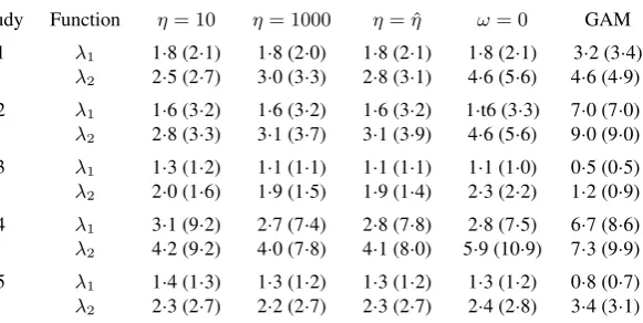
Table 1. Mean (×100) and standard deviation (×100) of the absolute difference between truth and posterior mean estimate for (λ1, λ2) in Studies 1 to 5 in Fig. 3 forη= (10,1000,ηˆ)andω= 0. The final column

refers to an estimated monotonized generalized additive model

Study Function η= 10 η= 1000 η= ˆη ω= 0 GAM

1 λ1 1·8 (2·1) 1·8 (2·0) 1·8 (2·1) 1·8 (2·1) 3·2 (3·4) λ2 2·5 (2·7) 3·0 (3·3) 2·8 (3·1) 4·6 (5·6) 4·6 (4·9)

2 λ1 1·6 (3·2) 1·6 (3·2) 1·6 (3·2) 1·t6 (3·3) 7·0 (7·0) λ2 2·8 (3·3) 3·1 (3·7) 3·1 (3·9) 4·6 (5·6) 9·0 (9·0)

3 λ1 1·3 (1·2) 1·1 (1·1) 1·1 (1·1) 1·1 (1·0) 0·5 (0·5) λ2 2·0 (1·6) 1·9 (1·5) 1·9 (1·4) 2·3 (2·2) 1·2 (0·9)

4 λ1 3·1 (9·2) 2·7 (7·4) 2·8 (7·8) 2·8 (7·5) 6·7 (8·6) λ2 4·2 (9·2) 4·0 (7·8) 4·1 (8·0) 5·9 (10·9) 7·3 (9·9)

5 λ1 1·4 (1·3) 1·3 (1·2) 1·3 (1·2) 1·3 (1·2) 0·8 (0·7) λ2 2·3 (2·7) 2·2 (2·7) 2·3 (2·7) 2·4 (2·8) 3·4 (3·1)

moves are proposed with probabilities 0·3, 0·3 and 0·4. Estimates for∆1, . . . ,∆Kare based on 275

3,000,000 iterations, with the first 1,000,000 discarded, and then every 1000th sample stored. Convergence of the sampled Markov chains for ∆_k (k= 1, . . . , K) is checked via the trace plots of λk(x) for ten random points in X. Posterior mean plots and trace plot examples are provided in the Supplementary Material. We also applied our methodology to non-Gaussian settings; an example with binomial response data is presented in the Supplementary Material. 280

The C++ and R code for all simulations is provided in the Supplementary Material.

3·2. Sensitivity analysis onη

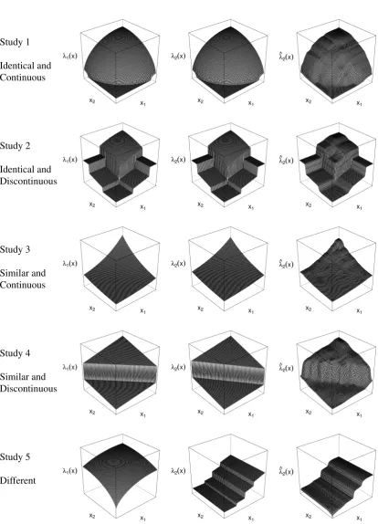
We explore general performance and sensitivity to η based on five simulations with K = 2 regions. Columns 1 and 2 in Fig. 3 illustrate the five pairs of (λ1, λ2). Across all studies, λk(xk)∈[0,2](k= 1,2). For each study, 1,000 and 100 data points are sampled for regions 1 285

and 2, respectively, withθk = 0·52 andxk∼Unif([0,1]2) (k= 1,2). This setting explores the potential benefits of borrowing statistical information from region 1 when estimatingλ2. We fix the prior parameterp= 1 and consider three settings forη: (i) η= 10, (ii)η = 1000and (iii) η= ˆη. Here,ηˆis the posterior mean estimate forηin the caseω= 0as described in§2·4.

We also estimate a monotonized generalized additive model for each region separately and 290

derive the same summary statistics as for our approach. We first fit a generalized additive model (Hastie & Tibshirani, 1990) and then apply the projection by Lin & Dunson (2014); plots of the estimated surfaces are provided in the Supplementary Material.

Study 1 and 2 consider the caseλ1=λ2 and Table 1 shows reduced error measures, partic-ularly for region 2, compared to the setting whenω= 0. Figure 3 illustrates that both smooth 295

surfaces and discontinuities are recovered well. In Study 3 and Study 4,λ1 andλ2 are similar and the conclusions are consistent with those for Study 1 and Study 2. Study 5 considers the case ofλ1 being smooth whileλ2 is piecewise linear. Table 1 shows no worsening in the error measures, demonstrating robustness of our methodology. The prospect of variable selection de-scribed in§2·3 has been examined forλ2in Study 5, whereλ2(x)depends only onx2,1. Almost 300

all sampled points are in∆_2,1, hence the results indicatex2,2to be redundant.

Study 1

Identical and Continuous

Study 2

Identical and Discontinuous

Study 3

Similar and Continuous

Study 4

Similar and Discontinuous

Study 5

Different

Fig. 3. True functions λ1 (Column 1) and λ2 (Column

2), and the posterior mean estimateλˆ2 obtained forη=

Fig. 4. True functions (λ1, λ2, λ3) in §3·3. The λk(x)

-axis (k= 1,2,3) is from 0 to 3.

Table 2. Mean (×100) and standard deviation (×100) of the abso-lute difference between the truth and posterior mean estimate for

(λ1, λ2, λ3)in Fig. 4 for the settingsp= (1·0,0·2,0·6,2·0)andω= 0

Study p= 1·0 p= 0·2 p= 0·6 p= 2·0 ω= 0

1 5·9 (8·3) 5·3 (7·9) 5·2 (7·4) 5·8 (8·5) 6·3 (9·3) 2 6·3 (9·5) 5·9 (10·0) 6·1 (10·0) 6·1 (10·1) 7·0 (11·9) 3 6·4 (8·8) 5·9 (9·0) 6·0 (9·1) 6·9 (9·7) 6·8 (9·6)

3, or requires a large number of points to be approximated, as in Study 4. Conversely,η= 10 305

performs better in Study 1 and Study 2, as it does not tend to interpolate linearly when functions switch between a zero and non-zero slope. These findings are consistent with§2: a higher value forηtends to produce smoother estimates, as the sampled functions have more but smaller steps.

3·3. Sensitivity analysis onp

We considerK= 3regions with region 2 adjacent to regions 1 and 3 while region 1 and 3 are 310

non-adjacent. Figure 4 shows the true functions (λ1, λ2, λ3), which all exhibit a discontinuity at (0·5,0·5), and are more similar for xk∈[0,1]2\[0·5,1·0]2 than for xk ∈[0·5,1·0]2 (k= 1,2,3). The distribution ofxk(k= 1,2,3) varies across three studies whileλ1, λ2andλ3remain unchanged. Specifically, the studies explore the performance of our approach, subject to the relative intensity of points in subsets ofXfor which the functions are similar. 315

We generate 200 data points for each region with varianceθk= 0·22(k= 1,2,3). The three studies vary with respect to the number of observations sampled on[0·5,1·0]2_{for regions 1 and 3} whilex2 ∼Unif([0,1]2)in all of them. Study 1 considers the casexk ∼Unif([0,1]2)(k= 1,3). In Study 2, 150 data points are sampled uniformly from[0·5,1·0]2 for regions 1 and 3, while only 25 observations are sampled from this subset in Study 3. The remaining 175 and 50 data 320

points in Study 2 and Study 3, respectively, are sampled uniformly from[0·0,1·0]2\[0·5,1·0]2. We compare four settings for p. The first,p= 1, yields the integrated squared difference in expression (2). Settingsp= 0·2andp= 0·6 allow for stronger dependence in the lower func-tion values, while p= 2 imposes increased dependence for higher function values. The other parameters are fixed toη= 1000,d1,2 =d2,3 = 1andd1,3= 0. 325

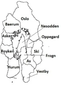
induc-Fig. 5. Map of the Norwegian municipalities in§4.

ing a large bias on the upper function values. As such, our extended discrepancy measure based

330

on (3) has benefits when compared to the integrated squared distance. Table 2 further indicates that the sensitivity topdepends on where most of the data are observed: if data fall in areas where the functions differ, the sensitivity is lower. The individual summary statistics for each function are provided in the Supplementary Material.

4. CASE STUDY

335

We consider the Norwegian insurance and weather data used by Haug et al. (2011) and Scheel et al. (2013). The data provide the daily number of insurance claims due to precipitation, surface water, snow melt, undermined drainage, sewage back-flow or blocked pipes at municipality level from 1997 to 2006. Further, the average number of policies held per month and multiple daily weather metrics, such as the amount of precipitation, are recorded.

340

Table 2 in Scheel et al. (2013) indicates that a generalized linear model underpredicts high numbers of claims, perhaps, due to threshold effects, as the risk of localized flooding only exists for high daily precipitation levels. While linearity may be too strong an assumption, the risk per property increases with precipitation levels, motivating the application of our methodology. We consider the K= 11 municipalities in Fig. 5 and explore the effect of precipitationRk,t and

345

Rk,t−1 (k= 1, . . . ,11) on daytandt−1, as Haug et al. (2011) and Scheel et al. (2013) find these to be the most informative explanatory variables.

LetNk,tandAk,tdenote the number of claims and policies, respectively, on daytfor munic-ipalityk. We modelNk,tas binomial with the logit of the daily claim probability,pk,t, given by λk(Rk,t, Rk,t−1). As in§3, we defineλk(Rk,t, Rk,t−1) =µk+ϕk(Rk,t, Rk,t−1)and estimate

350

µkandϕk(k= 1, . . . ,11). Formally,

Nk,t ∼Binomial(Ak,t, pk,t), logitpk,t=µk+ϕk(Rk,t, Rk,t−1).

An intrinsic conditional autoregressive prior is defined for µ1, . . . , µ11, and the boundaries of ϕk(k= 1, . . . ,11) are set toδmin= 0andδmax= 10. The setXis derived as the square spanned by the observed minima and maxima ofRk,tacross all municipalities and years.

We setdk,k0 = 1in (4) if municipalitieskandk0are adjacent andd_k,k0 = 0otherwise. To avoid 355

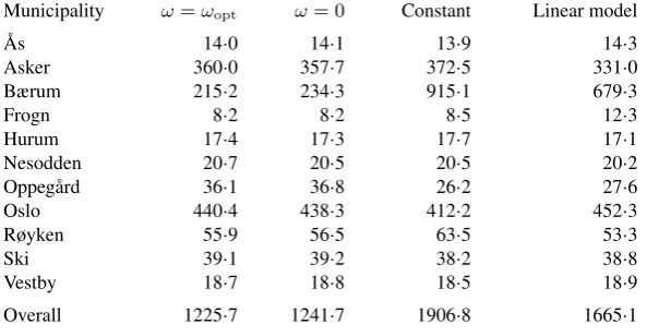
vul-Table 3.Sum of squared errors of the daily number of claims for 2001 and 2003 for four models with estimates being based on the remaining

8 years between 1997 and 2006

Municipality ω=ωopt ω= 0 Constant Linear model

˚

As 14·0 14·1 13·9 14·3

Asker 360·0 357·7 372·5 331·0

Bærum 215·2 234·3 915·1 679·3

Frogn 8·2 8·2 8·5 12·3

Hurum 17·4 17·3 17·7 17·1

Nesodden 20·7 20·5 20·5 20·2

Oppeg˚ard 36·1 36·8 26·2 27·6

Oslo 440·4 438·3 412·2 452·3

Røyken 55·9 56·5 63·5 53·3

Ski 39·1 39·2 38·2 38·8

Vestby 18·7 18·8 18·5 18·9

Overall 1225·7 1241·7 1906·8 1665·1

nerability to small amounts of precipitation, while differences in infrastructure, for example, may lead to different effects for higher precipitation levels. We setp= 0·5. The functionsλ1, . . . , λ11 are estimated based on 1,000,000 iteration steps,with every 500th sample stored after a burn-in 360

period of 200,000 iterations.

To assess predictive performance, observations for 2001 and 2003 are stored as test data and λ1, . . . , λ11are estimated from the remaining eight years. We consider two competing models: (i) the average daily number of claims in the municipality over the training period and (ii) a linear model with spatially varying parameters (Assunc¸˜ao, 2003). The latter is estimated via 10,000 365

iterations of a random walk Metropolis scheme, with the first 1,000 samples discarded.

Table 3 shows that our approach is the best in terms of overall predictive performance. The small scale of improvement fromω = 0toω=ωopt is due to the large number of training data points; important structures inλ1, . . . , λ11are likely to be captured without borrowing statistical information from adjacent municipalities. Posterior mean plots for Oslo and Hurum are provided 370

in the Supplementary Material, but the function values are omitted for confidentiality reasons. The largest improvement is achieved for Bærum, which has the highestNk,tover the test pe-riod. Hence, the increased flexibility of our approach captures the dynamics leading to large num-bers of claims better than competing models. For the other municipalities, the models perform similarly, due to there being zero high-claim days over the test period. This is also indicated by 375

the predictive error of the constant mean model being low for most municipalities. Our approach performs slightly worse than the linear model for Asker, which is due to a single observation Nk,t. In particular, high precipitation levels caused a countNk,twhich was the highest over the full 10-year period.

5. DISCUSSION 380

Our modelling framework can be extended to a spatio-temporal context. Assume that the in-tercept changes between observations but the effect of the explanatory variables is temporally stationary. We can then define λk,t(x) =µk,t+ϕk(x) (k= 1, . . . , K), similar to §3 and §4. Temporal structure onµk,1, . . . , µk,Tkis, for instance, imposed via an autoregressive model. Our

approach can also be extended to a setting for whichλ1, . . . , λKchange at specified time points, 385

An aspect not discussed is the selection of the numberIof marked point processes represent-ingλk(k= 1, . . . , K). Since we considered examples withm= 2explanatory variables,I = 3. In higher dimensions, however, one may want to restrictI. Assume there exists prior knowledge that continuous variablexk,h(h= 1, . . . , m) is informative and letX= [0,1]m. The set of

pro-390

cesses could then be defined based on the non-empty subsets of {1, . . . , m}which contain h. Consequently, we would representλk(k= 1. . . , K) via2m−1, instead of2m−1, processes.

Our methodology performs well for regression problems withm= 2tom= 5 explanatory variables. However, as for other flexible approaches, such as generalized additive models, some issues arise for higher dimensions. Firstly, the computational cost for calculating the prior ratio

395

grows exponentially withm. We reduce this cost by deriving the subset ofX affected by the proposal before evaluating the integral in expression (4). Secondly, the monotonicity constraint becomes less restrictive with increasing dimension, leading to potential overfitting. Larger sets of explanatory variables can be accommodated by imposing an additive or semi-parametric struc-ture onλk(k= 1, . . . , K), where the lower-dimensional monotonic functions are then estimated

400

jointly. Consequently, our methodology can be applied to higher-dimensional regression prob-lems, but we would recommend a pre-analysis.

Our work can be extended in several ways, such as the construction of other discrepancy mea-sures based, for instance, on the Kullback–Leibler divergence. When estimatingω, parallelized computing techniques, allocating the folds to multiple processors, can reduce the computational

405

time. Further, we arbitrarily fixed the number of folds tos= 10but the value forωalso depends on the number of data points. A larger number of folds may return a more robust estimate.

ACKNOWLEDGEMENT

Rohrbeck gratefully acknowledges funding by the EPSRC via the STOR-i Centre for Doc-toral Training. This paper was also financially supported by the Norwegian Research Council.

410

Our work greatly benefited from discussions with Jonathan Tawn, Paul Fearnhead, Elija Arjas, Christopher Nemeth, Sylvia Richardson, Lawrence Bardwell, Jamie Fairbrother, David Hofmeyr, Rob Shooter, Jennifer Wadsworth and Ida Scheel. We also thank Ida Scheel for providing access to the insurance and weather data. Finally, we would like to thank the editors and two referees for suggestions that substantially improved the presentation of the work.

415

SUPPLEMENTARY MATERIAL

Supplementary material available onBiometrikaonline contains a dependence model for func-tions with varying support, details on the prior and the sampling scheme, the proofs of Propo-sition 1 and Theorem 1, an algorithm to detect discontinuities, a simulation study to verify cor-rectness of our implementation, posterior mean plots, trace plots to illustrate mixing and

conver-420

gence, an example with binomial response data, data plots and posterior mean estimates for two municipalities of the case study, and the C++ and R code for§3.

APPENDIX

Details of the sampling scheme for the marked point processes

We present the acceptance probabilities for the three moves in§2·5; more details are provided in the

425

A birth move proposes the addition of a point(ξ∗, δ∗)to∆k,i∗. Since this increases the dimension

of the parameter space, the acceptance probability has to be derived as described by Green (1995). The mapping for adding a point is equal to the identity function and, hence, the determinant of the Jacobian in 430

the acceptance probability is equal to 1. Further, the proposal densitiesq(ξ∗_)andq(δ∗_|ξ∗_,∆

k)cancel

with parts of the priorφ(∆k|η). Formally, the acceptance probability is

min    1, Tk Y t=1

f{yk,t|λ∗k(xk,t), θk}

f{yk,t|λk(xk,t), θk}

× Y

k0_6=k

exp−ω dk,k0 R

Xγp

_˜

λ∗_k(x),λ˜k0(x) dx

exp−ω dk,k0 R

Xγp

_˜

λk(x),˜λk0(x) dx

×

1−1 η

_N

k+ 1

Nk+I

 



.

A death or shift move is rejected if∆k,i∗ contains no points. Otherwise, a death move selects one of

thenk,i∗existing points with equal probability and proposes to remove it. The acceptance probability for

a death move is then 435

min    1, Tk Y t=1

fyk,t|λ˜∗k(xk,t), θk

f

yk,t|λ˜k(xk,t), θk

× Y

k0_6=k

exp−ω dk,k0 R

Xγp

_˜

λ∗

k(x),λ˜k0(x) dx

exp

−ω dk,k0 R

Xγp

_˜

λk(x),λ˜k0(x) dx

× 1

1−1

η

Nk+I−1

Nk

 



.

Finally, a shift move changes both the location and mark of an existing point, subject to the partial ordering of the locations in∆k,1. . . ,∆k,I, induced by the monotonicity constraint, being maintained.

First, one of thenk,i∗points in∆_k,i∗is selected with equal probability. The proposed locationξ∗is then

sampled uniformly on the subset ofXiwhich maintains the total order in each component of the locations;

see Saarela & Arjas (2011) for details. The proposed markδ∗ is then sampled uniformly, subject to the 440

monotonicity constraints. Formally, the acceptance probability is

min    1, Tk Y t=1

fyk,t|˜λk(xk,t), θk

f

yk,t|˜λk(xk,t), θk

× Y

k0_6=k

exp−ω dk,k0 R

Xγp

_˜

λk(x),˜λk0(x) dx

exp−ω dk,k0 R

Xγp

_˜

λk(x),˜λk0(x) dx

 



.

REFERENCES

ANDRIEU, C. & ROBERTS, G. O. (2009). The pseudo-marginal approach for efficient Monte Carlo computations. Ann. Statist.37, 697–725.

ASSUNC¸ ˜AO, R. M. (2003). Space varying coefficient models for small area data.Environmetrics14, 453–473. 445

AYER, M., BRUNK, H. D., EWING, G. M., REID, W. T. & SILVERMAN, E. (1955). An empirical distribution function for sampling with incomplete information.Ann. Math. Statist.26, 641–647.

BACCHETTI, P. (1989). Additive isotonic model.J. Am. Statist. Assoc.84, 289–294.

BARLOW, R. & BRUNK, H. (1972). The isotonic regression problem and its dual.J. Am. Statist. Assoc.67, 140–147. BARRON, A., SCHERVISH, M. J. & WASSERMAN, L. (1999). The consistency of posterior distributions in nonpara- 450

metric problems.Ann. Statist.27, 536–561.

BEAUMONT, M. A., ZHANG, W. & BALDING, D. J. (2002). Approximate Bayesian computation in population genetics. Genetics162, 2025–2035.

BELL, M. L., MCDERMOTT, A., ZEGER, S. L., SAMET, J. M. & DOMINICI, F. (2004). Ozone and short-term mortality in 95 US urban communities, 1987–2000.J. Am. Med. Assoc.292, 2372–2378. 455

BERGERSEN, L. C., THARMARATNAM, K. & GLAD, I. K. (2014). Monotone splines lasso. Comp. Statist. Data Anal.77, 336–351.

BESAG, J., YORK, J. & MOLLIE´, A. (1991). Bayesian image restoration, with two applications in spatial statistics. Ann. Inst. Statist. Math.43, 1–20.

BOWMAN, A. W. & AZZALINI, A. (1997).Applied Smoothing Techniques for Data Analysis: The Kernel Approach 460 with S-Plus Illustrations. Oxford: Clarendon Press.

BOWMAN, A. W., JONES, M. C. & GIJBELS, I. (1998). Testing monotonicity of regression.J. Comp. Graph. Statist. 7, 489–500.

BRUNK, H. D. (1955). Maximum likelihood estimates of monotone parameters.Ann. Math. Statist.26, 607–616. BRUNK, H. D., EWING, G. M. & UTZ, W. R. (1957). Minimizing integrals in certain classes of monotone functions. 465

Pacific J. Math.7, 833–847.

CAHILL, M. & MULLIGAN, G. (2007). Using geographically weighted regression to explore local crime patterns. Social Science Computer Review25, 174–193.

CONGDON, P. (2006). A model for non-parametric spatially varying regression effects. Comp. Statist. Data Anal.

FANG, Z. & MEINSHAUSEN, N. (2012). LASSO isotone for high-dimensional additive isotonic regression.J. Comp. Graph. Statist.21, 72–91.

FARAH, M., KOTTAS, A. & MORRIS, R. D. (2013). An application of semiparametric Bayesian isotonic regression to the study of radiation effects in spaceborne microelectronics.Appl. Statist.62, 3–24.

FOTHERINGHAM, A. S., BRUNSDON, C. & CHARLTON, M. (2003).Geographically weighted regression: the anal-475

ysis of spatially varying relationships. Hoboken, NJ: Wiley.

GELFAND, A. E. & KUO, L. (1991). Nonparametric Bayesian bioassay including ordered polytomous response. Biometrika78, 657–666.

GEORGII, H.-O. (2011).Gibbs Measures and Phase Transitions. Berlin: de Gruyter, 2nd ed.

GHOSAL, S., SEN, A. &VAN DER VAART, A. W. (2000). Testing monotonicity of regression. Ann. Statist.28,

480

1054–1082.

GREEN, P. J. (1995). Reversible jump Markov chain Monte Carlo computation and Bayesian model determination. Biometrika82, 711–732.

HASTIE, T. J. & TIBSHIRANI, R. J. (1990).Generalized Additive Models. Boca Raton, Fla.: Chapman & Hall. HAUG, O., DIMAKOS, X. K., V ˚ARDAL, F., J., ALDRIN, M. & MEZE-HAUSKEN, E. (2011). Future building water

485

loss projections posed by climate change.Scandinavian Actuarial Journal2011, 1–20.

HEIKKINEN, J. & ARJAS, E. (1998). Non-parametric Bayesian estimation of a spatial Poisson intensity. Scand. J. Statist.25, 435–450.

JONES, D. R., SCHONLAU, M. & WELCH, W. J. (1998). Efficient global optimization of expensive black-box functions.Journal of Global Optimization13, 455–492.

490

KNORR-HELD, L. (2003). Some remarks on Gaussian Markov random field models for disease mapping. InHighly Structured Stochastic Systems, P. J. Green, N. L. Hjort & S. Richardson, eds. Oxford: Oxford University Press, pp. 203–207.

LIN, L. & DUNSON, D. B. (2014). Bayesian monotone regression using Gaussian process projection. Biometrika, 303–317.

495

LUSS, R., ROSSET, S. & SHAHAR, M. (2012). Efficient regularized isotonic regression with application to gene– gene interaction search.Ann. Appl. Statist.6, 253–283.

MØLLER, J., PETTITT, A. N., REEVES, R. & BERTHELSEN, K. K. (2006). An efficient Markov chain Monte Carlo method for distributions with intractable normalising constants.Biometrika93, 451–458.

PENTTINEN, A., STOYAN, D. & HENTTONEN, H. M. (1992). Marked point processes in forest statistics. Forest 500

Science38, 806–824.

RAMSAY, J. O. (1998). Estimating smooth monotone functions.J. R. Statist. Soc. B60, 365–375. RAMSAY, J. O. & SILVERMAN, B. W. (2005).Functional Data Analysis. New York: Springer, 2nd ed.

ROUSTANT, O., GINSBOURGER, D. & DEVILLE, Y. (2012). DiceKriging, DiceOptim: Two R packages for the analysis of computer experiments by kriging-based metamodeling and optimization.J. Statist. Softw.51, 1–55.

505

ROYSTON, P. (2000). A useful monotonic non-linear model with applications in medicine and epidemiology.Statist. Med.19, 2053–2066.

RUE, H. & HELD, L. (2005).Gaussian Markov Random Fields: Theory and Applications. Boca Raton, Fla.: Chap-man & Hall.

SAARELA, O. & ARJAS, E. (2011). A method for Bayesian monotonic multiple regression. Scand. J. Statist.38,

510

499–513.

SCHEEL, I., FERKINGSTAD, E., FRIGESSI, A., HAUG, O., HINNERICHSEN, M. & MEZE-HAUSKEN, E. (2013). A Bayesian hierarchical model with spatial variable selection: The effect of weather on insurance claims. Appl. Statist.62, 85–100.

SCOTT, J. G., SHIVELY, T. S. & WALKER, S. G. (2015). Nonparametric Bayesian testing for monotonicity.

515

Biometrika102, 617–630.

SHIVELY, T. S., SAGER, T. W. & WALKER, S. G. (2009). A Bayesian approach to non-parametric monotone function estimation.J. R. Statist. Soc. B71, 159–175.

TUTZ, G. & LEITENSTORFER, F. (2007). Generalized smooth monotonic regression in additive modeling.J. Comp. Graph. Statist.16, 165–188.

520

WAKEFIELD, J. (2007). Disease mapping and spatial regression with count data.Biostatistics8, 158–183. WALKER, S. G. & HJORT, N. L. (2001). On Bayesian consistency.J. R. Statist. Soc. B63, 811–821.

WALLER, L. A. & GOTWAY, C. A. (2004).Applied Spatial Statistics for Public Health Data. Hoboken, NJ: Wiley. WILSON, A., REIF, D. M. & REICH, B. J. (2014). Hierarchical dose–response modeling for high-throughput toxicity

screening of environmental chemicals.Biometrics70, 237–246.

525

ZHANG, L. & SHI, H. (2004). Local modeling of tree growth by geographically weighted regression.Forest Science 50, 225–244.