A structural accounting framework
for estimating the expected rate of return on equity
Demetris Christodoulou
∗Colin Clubb
Stuart McLeay
Version: October 19, 2015
∗The authors are, respectively, at The University of Sydney, King’s College London and Lancaster University. We
A structural accounting framework
for estimating the expected rate of return on equity
Abstract
This paper shows how the expected rate of return (ERR) on equity may be estimated using published
accounting results, based on the information dynamics of reported earnings. As accounting-based
valua-tion models condivalua-tional upon financial statement articulavalua-tion lead to a rank deficient system of estimating
equations, the paper introduces a nonlinear constraint on the articulation that allows the information
system simultaneously to produce an estimate for the ERR by iteration, together with predictions for the
key clean surplus forecasts of net earnings, net dividend and the book value of equity. Further
decompo-sition produces estimates of expected capital gain, expected earnings and the expected change in equity
book value, and by rearrangement, the expected change in unrecorded goodwill. The clean surplus
rela-tion is maintained in the forecast variables. Exploratory data methods are used to examine the nonlinear
relationship between components of the accounting-based ERR and realized stock returns. Findings show
that realized returns are higher (lower) than estimated ERR in expansionary (recessionary) periods, with
evidence of a stronger returns impact in recessionary periods. For the large majority of firms, realized
returns revert to the estimated ERR, and the time-varying accounting components are strongly related
to future realized stock returns, consistent with time variation in the ERR around a long-run average.
Predicted earnings and dividends provide useful additional information on short-run variations in the
ERR.
1
Introduction
This paper is concerned with using only key accounting information to estimate the firm’s long-run rate
of return on its equity. Our analysis differs from previous research by focusing on how information
dynamics can be adapted in order to estimate the expected return using published accounting data, in
marked contrast to most of the extant accounting literature which reverse-engineers the expected return
using using earnings forecasts and stock prices.
We apply theClubb(2013) development of theOhlson(1995) linear information dynamics framework
based on abnormal earnings (residual income) to extract an estimate of the firm’s expected rate of return.
In order to obtain estimates of the cost of equity under this approach, we convert the abnormal earnings
information dynamics into a reported earnings information dynamics and then, following the methods
proposed byChristodoulou and McLeay(2014), we introduce a constraint on accounting articulation into
the resulting rank deficient equation system, which is then estimated on a firm-by-firm basis.
The linear information system simultaneously produces an estimate for the expected return together
with predictions for future earnings, net dividend and closing book value of equity. We then apply
the Easton, Harris, and Ohlson (1992) and Penman and Yehuda(2009) decomposition of stock returns
to produce an estimate of expected change in price and employ exploratory data methods to examine
the non-linear relationship between components of our accounting-based expected return estimates and
realized stock returns.
The remainder of the paper is organized as follows. Section 2 reviews the relevant literature on
the use of accounting information to estimate expected returns. Section 3 develops the framework for
estimating and analysing the long-run expected rate of return and explains the estimation issues related
to implementation of this framework. Section 4 describes the data. Section 5 presents the results and
Section 6concludes.
2
Accounting information and expected returns
The relationship between the expected rate of return (ERR) on equity and information about the firm’s
fundamental economic performance and financial position is a considerably active area of theoretical and
empirical research in finance and accounting. Some of this substantial literature is reviewed in papers by
Callen(2016),Easton and Monahan(2016) andPenman(2016) in the current issue of this journal, so we
limit ourselves here to reviewing only those aspects of the literature that motivate and locate the analysis
in the current paper. Indeed, where possible, we exploit insights from these papers to highlight strengths
and limitations of the approach to estimating expected equity returns adopted in our study. At the
risk of over-simplification, we distinguish between ‘finance’ and ‘accounting’ perspectives in the literature
on ERR in this section. We start by briefly outlining some important developments from the ‘finance
perspective’ before focusing on issues raised by the ‘accounting perspective’ of particular relevance to our
analysis.
The ‘finance perspective’ on ERR is focused on the development of asset pricing models to provide
the-oretical and empirical insights into the drivers of expected returns. In relation to the role of fundamental
information, the seminal empirical studies by Fama and French(1992,1993) highlighted the possibility
of accounting information contributing to the identification of priced risk factors, in particular through
the book-to-market factor. However, as indicated by Easton and Monahan (2016) in this issue and as
such as the book-to-market and firm size as related to risk is somewhat controversial and lacks
unambigu-ous theoretical backing. More recent asset pricing research, on the other hand, has provided important
insight into why fundamentals-based variables, such as book-to-market, may be relevant for forecasting
expected returns. Notably, Campbell and Vuolteenaho (2004) and Campbell, Polk, and Vuolteenaho
(2009), building on previous theoretical work byCampbell(1991,1993) on stock return variance
decom-position and inter-temporal asset pricing, provide evidence to support the breakdown of the traditional
CAPM beta into four components representing the covariance of firm-level returns (decomposed into
cash flow news and discount rate news) with market returns (similarly decomposed into cash flow and
discount rate news). Their analysis suggests that beta based on the covariance of a firm’s stock returns
with market cash flow news (referred to as ‘bad beta’) should be, and appears to be, more highly priced
than beta based on the covariance of a firm’s stock returns with market discount rate news (referred to
as ‘good beta’). Their results show that value stocks (with high book-to-market ratios) have had higher
bad beta and lower good beta compared to growth stocks (with low book-to-market) since the 1960’s,
helping to explain the apparently anomalous higher average returns of value stocks during this period.
Research taking the ‘finance perspective’, such as that based on extensions of the CAPM alluded to
above, not only indicates how asset pricing theory can explain the usefulness of accounting-based variables
such as book-to-market for forecasting expected returns; perhaps more importantly, this research also
makes use of accounting information in the measurement of risk. Campbell and Vuolteenaho(2004) and
Campbell et al.(2009) make use of firm-level and market-level VAR models which combine stock return
and accounting based data (specifically, book-to-market and accounting return on equity) to estimate cash
flow news and discount rate news components of unexpected returns. In other words, income statement
and balance sheet data play a major role in the decomposition of a firm’s systematic risk in their analysis.
Nevertheless, whilst making extensive use of accounting data to estimate beta risk components, the
‘finance perspective’ ultimately focuses on cash payoffs to investors and does not explicitly highlight
conceptual issues in relation to the role of accounting information in predicting the amount, timing and
riskiness of future firm cash flows.
The ‘accounting perspective’ on ERR emphasizes how accounting converts cash flow data into earnings
and book values, which can then be used to assess the riskiness of a firm’s operations and/or forecast
future expected stock returns. An important ingredient in most accounting studies of expected returns
(including the current paper) is the so-called ‘clean surplus relation’ (CSR) which links net dividends paid
out to investors to accounting earnings and book value of equity. For example,Penman(2016) utilizes the
CSR to analyze the possible role of earnings-to-price as an indicator of firm risk, while also arguing that
the accounting ‘structure must communicate risk that results in a discount to the denominating price
(in the earnings-to-price ratio) to yield a higher expected return that reflects that risk’. Penman(2016)
therefore argues for the need to go beyond the limited structure given to accounting by the CSR to gain
an understanding of how accounting practices based on the risk-related deferral of income may generate
information relevant to the assessment of firm risk. His analysis also highlights a growing empirical
literature which investigates accounting information from this perspective and which broadly confirms
the expectation that future realized stock returns are higher and riskier (both in terms of volatility and
sensitivity to market movements) for firms with higher earnings growth related to earnings deferrals under
conservative accounting.
As highlighted byEaston and Monahan(2016) andCallen(2016), there is also a substantial literature
from the ‘accounting perspective’ which uses the residual income valuation model based on the CSR to
reverse-engineer ERRs from stock prices or to analyze time variation in ERRs. Whilst the empirical
theoretical analysis ofCampbell(1999) andVuolteenaho(2002) (and with research based on the ‘finance
perspective’ previously discussed), the large literature on estimation of implied cost of capital’ reviewed
by Easton and Monahan (2016) indicates the continued importance of the simple constant discount
rate model both for equity valuation and for management investment decision-making. The accounting
perspective on expected stock returns in the current paper is consistent with the focus in the implied
cost of capital literature on estimating an average or long-run expected rate of return. There are however
also some important differences between our approach to ERR estimation and other approaches in the
literature which we now briefly summarize before moving to a detailed outline of our research design.
The framework for estimating ERR adopted in the remainder of this paper aims to contribute to
the ‘accounting perspective’ on ERR estimation and fundamental performance. More specifically, we
use the linear information model based on abnormal earnings, net dividend, and book value of equity
from Clubb (2013) to estimate the long-run expected return on equity on a firm-by-firm basis. This is
achieved by replacing abnormal earnings with net earnings less lagged book value multiplied by ERR
in the information dynamics; applying the CSR parameter constraints identified in Clubb(2013) to the
adjusted dynamics; and applying estimation methods to deal with rank deficiency of the resulting equation
system as in Christodoulou and McLeay (2014). This approach allows us to estimate a long-run ERR
based purely on the firm’s accounting information dynamics and without reference to its stock price, thus
avoiding the circularity problem of using reverse-engineered implied cost of capital estimates for equity
valuation noted byPenman(2016) in this issue.
Furthermore, as discussed more fully in Section3, theClubb(2013) dynamics is based on a
generaliza-tion of the dynamics used in the seminal work of Ohlson(1995) andFeltham and Ohlson (1995), which
facilitates understanding of implicit assumptions regarding dividend displacement and accounting
conser-vatism in our analysis. There are of course some potential limitations associated with our approach. For
example, we make simplified assumptions in relation to the information dynamics generating abnormal
earnings (in particular, we define abnormal earnings in relation to a risk-adjusted discount rate of return,
as opposed to the risk-free rate as advocated in research reviewed byCallen(2016)) and we do not provide
an explicit risk-based explanation of our long-run ERR estimates. However, we believe that our focus on
estimating the expected rate of return from linear information dynamics based on accounting
fundamen-tals represents a novel approach which highlights the possibility of focusing on a firm’s performance in
its product markets, as opposed to the capital market, to derive ERR estimates.
3
Structural estimation framework
This section begins with an outline of how accounting information models based on abnormal earnings
are to extract estimates of the expected rate of return on equity. After providing key definitions for
the clean surplus relation, we explain the rationale for our approach to ERR estimation by relating
accounting information dynamics to the key valuation concepts of unbiased and conservative accounting.
Second, we show how the assumed accounting information dynamics can be used not only to estimate
the ERR but also to forecast the key components of the ERR, including forecast earnings. Third, the
econometric issues related to the estimation of the accounting information dynamics and the implied
3.1
Clean surplus definitions
Clean surplus accounting prescribes the updating of the closing shareholders’ equity positionyt+1, given
the opening positionytplus the intervening period net earningsxt+1minus the net dividend distribution
to shareholdersdt+1:
yit+1≡xit+1−dit+1+yit. (1)
Specifically,xitis defined as clean surplus comprehensive net earnings of firmiat timet,ditis dividend
payout plus stock repurchases net of proceeds from new share issues, andyitis book value of equity. The
clean surplus relation can be re-expressed in terms of abnormal earnings, i.e. the difference between
reported net earnings and the equity capital charge given the knowledge of the expected rate of return,
xa
it+1=xit+1−riyit:
yit+1≡xait+1−dit+1+ (ri+ 1)yit, (2)
whereriis expected rate of return (the ERR) for firmi, which is assumed here to be inter-temporally
constant over the firm-specific time periodTi.
3.2
Abnormal earnings valuation, accounting bias and the ERR
The seminal studies byOhlson(1995) andFeltham and Ohlson(1995) demonstrate how linear information
dynamics can be used to derive equity values which exhibit a long-run expected value either equal to book
value (unbiased accounting) or in excess of book value (conservative accounting). In other words, these
studies demonstrate how linear information dynamics can be used to model the joint impact of product
market competition and accounting practices on the relationship between the long-run accounting rate of
return (ARR) and the ERR, where unbiased accounting implies long-run convergence of the ARR to the
ERR and conservative accounting implies long-run convergence of the ARR to a rate above the ERR.
In the case of unbiased accounting inOhlson(1995), long-run reversion of the accounting rate of return
to the ERR implies that abnormal earnings persistence,ω, is less than 1 in the following autoregression
of abnormal earnings:1
xait+1=ωxait+it+1, (3)
where it+1 is a mean zero Normal disturbance term. Given that 0 ≤ ω < 1, this model can be
viewed as consistent with competitive product markets where the economic rate of return generated by
the firm converges to the ERR in the long-run, and cost-based accounting valuation practices ensure that
the long-run ARR closely approximates this long-run economic rate of return. Furthermore, equation3
implies the following comprehensive earnings dynamic:
1The originalOhlson(1995) analysis also allowed for ‘other information’ variables, v
t, which are assumed byOhlson
xit+1=ωxit+riyit−ωriyit−1+it+1. (4)
Hence it follows that the ERR, ri, can be estimated as a composite coefficient on yit−1, via the
autoregression of net earnings, augmented by equity book value att, and lagged book value att−1.
The information dynamics represented by equations3and4may not represent useful earnings forecast
models for firms that operate in imperfectly competitive product markets and/or implement accounting
valuation procedures that systematically value assets below cost. Such conditions where the long-run
ARR is expected to be above the ERR are modelled by Feltham and Ohlson (1995), who assume the
following abnormal earnings dynamic:
xait+1=ωxait+γyit+it+1, (5)
where 0 ≤ω <1 andγ > 0. Given that book value is expected to grow at a positive rate (i.e. it is
not mean-reverting), then γ > 0 implies non-convergence of abnormal earnings to zero in the long-run,
which in turn implies ‘accounting conservatism’ where abnormal earnings are positive and expected ARR
is greater than ERR. Extraction of the ERR from the Feltham and Ohlson(1995) model is based on:
xit+1=ωxit+ (ri+γ)yit−ωriyit−1+it+1, (6)
where the ERR may be inferred from the regression coefficients for comprehensive earnings at t and
book value of equity at date t−1 based on equation6.
WhileFeltham and Ohlson(1995) provides one approach to modeling conservative accounting based
on linear accounting information dynamics, a controversial feature of the implied equity valuation
func-tion is that a marginal dollar increase in net dividends reduces equity value by more than a dollar, i.e.
that dividend displacement does not hold and net dividends turn out to be a negative indicator of value
as a result of the assumption that γ > 0. An alternative approach to modeling conservative
account-ing highlighted by Pope and Wang (2005) and Clubb (2013), which is consistent with the Miller and
Modigliani(1961) dividend displacement property, is to assume that abnormal earnings are generated by
the following dynamic process:
xait+1=ωxait+φdit+it+1, (7)
where the assumption that φ >0 implies accounting conservatism, i.e. a long-run ARR above the
ERR. The corresponding comprehensive earnings dynamic is:
xit+1=ωxit+φdit+riyit−ωriyit−1+it+1, (8)
estimation of long-run expected return on equity under the assumption that long-run ARR may exceed
ERR, and avoids the implication of theFeltham and Ohlson(1995) model that net dividends reducecum
div equity value, we use equation8in our empirical analysis to estimate the ERR, as discussed below.
3.3
Estimation model
Our analysis employs the following linear information dynamics fromClubb(2013):2
xait+1=α1+ω11xait+ω12dit+1it+1 (9a)
dit+1=α2+ω21xait+ω22dit+ω23yit+2it+1 (9b)
yit+1=α3+ω31xait+ω32dit+ω33yit+3it+1 , (9c)
All error terms are assumed to be Normal mean zero disturbances. The estimation of the system of
equations 9a - 9c requires knowledge of the rate of return on equity ri in order to measure abnormal
earnings,xa
it+1=xit+1−riyit. However, rewriting the system in terms of reported earnings obviates the need to know ri, which instead can be estimated as a free parameter using the restricted least squares
approach fromChristodoulou and McLeay(2014):
xit+1=α1+ω11xit+ω12dit+riyit−ω11riyit−1+1it+1 (10a)
dit+1=α2+ω21xit+ω22dit+ω23yit−ω21riyit−1+2it+1 (10b)
yit+1=α3+ω31xit+ω32dit+ω33yit−ω31riyit−1+3it+1 , (10c)
Note that equation 10a corresponds exactly to equation 8. Since earnings are measured on a clean
surplus basis, as described in Section 3.1, Clubb (2013) notes that the linear information system of
equations10a -10cimplies that the following parameter restrictions must hold:
α3=α1−α2 (11a)
ω31=ω11−ω21 (11b)
ω32=ω12−ω22 (11c)
ω33= (ri+ 1)−ω23. (11d)
The linear information system described above is a rank deficient system of seemingly unrelated
re-gressions. The system is characterized by a singular variance-covariance (VCE) matrix because it holds
that 0 +E(1it+1)−E(2it+1) =E(3it+1); the inclusion of zero emphasizes that opening equity has zero
residual because it is known and conforms with the clean surplus identity ofyit≡xit−dit+yit−1. Greene
and Seaks(1991) andGreene(2011) explain how such rank deficient systems can be estimated in one of
two ways. We may impose the parameter restrictions of equations11a -11dand estimate the system of
equations 10a -10cvia restricted least squares with the singular VCE. Alternatively, unrestricted least
2The linear information dynamics may be extended to include other value relevant information given the valuation
squares can be applied to recover the estimates of two out of three equations, and then the estimates of
the third equation are deduced from the known relationship between parameters. In this case, given the
model, the predetermined opening equity yit and the predicted ˆxit+1 and ˆdit+1, then the predicted
clos-ing equity ˆyit+1 is simply deduced by means of the structural requirement of the clean surplus condition
governing the accounting variables that are forecasted:3
yit+ ˆxit+1−dˆit+1≡yˆit+1 . (12)
This articulation of predictions makes it clear that it is only necessary to estimate two out of three
equations from the rank deficient system of linear information dynamics in equations10a-10c. Equation
12can also be expressed in terms of abnormal earnings, without needing to predict abnormal returns as
intended in the original linear information dynamics:
(1 + ˆri)yit+ ˆxait+1−dˆit+1≡yˆit+1 . (13)
The individual predictions are analysed in detail in Section5. The system of accounting information
dynamics is not only rank deficient in its equations, but also contains rank deficient design matrices
X, and the common presence ofri places additional cross-equation restrictions in non-linear estimation.
These econometric implications are discussed further in Section3.5.
3.4
ERR structure
Given an estimate for ˆrifrom equations10a-10c, it is possible to use the relationship between observed
stock returns and accounting earnings from Easton et al. (1992) and Penman and Yehuda (2009) to
separate ˆri into forecast components for the expected earnings yield, the expected percentage change
in market value of equity, and the expected change in book value to equity with respect to its current
market value, where the decomposition follows from the clean surplus identity of equation1:
ˆ
ri= ˆ
pit+1−pit pit
+ ˆ
dit+1 pit
= xˆit+1
pit
+pˆit+1−pit
pit
−yˆit+1−yit
pit
, (14)
where ˆ denotes predictions formed att fort+ 1, ˆri is a parameter estimate from the linear information
dynamics of equations 10a - 10c, ˆxit+1/pit, ˆdit+1/pit and ˆyit+1/pit are the articulated predictions for
reported earnings, net dividend and book value of equity, respectively, and pit is market value of equity.
The decomposition in equation14reflects theEaston et al.(1992) proposition that the expected return is
driven by expected earnings adjusted for the change in expected unrecorded goodwill, as represented by
the two last terms in equation14. Note that the last term representing expected capital gain is estimated
simply by rearranging the equation as follows:
3Greene(2011) discusses rank deficient systems of equations, explaining how the estimation ofK−1 equations is sufficient
ˆ
pit+1−pit pit
= ˆri− ˆ
xit+1 pit
−yˆit+1−yit
pit
. (15)
3.5
Restricted non-linear least squares
The estimation model given by equations 10a - 10c is non-linear in its parameters and is estimated
via iterative generalized non-linear least squares (IFGNLS), which is equivalent to maximum likelihood
estimation (MLE) with multivariate normal disturbances across equations. It is important to iterate
towards convergence to MLE, because the solution is invariant to choosing to estimate two out of three
equations. As mentioned in Section 3.3, the third can be deduced using the parameter relations in
equations11a-11d, given the known opening equity and the singular system of linear information dynamics
for clean surplus items.
The stacked system of equations represents a seemingly unrelated regression (SUR) estimator. In
the absence of an integrated system, the SUR estimator makes the assumption of cross-equation error
correlation for theitthobervation,E(1it+1, 2it+1)6= 0, and produces more efficient estimates than simple
NLS when the equations are non-identical and non-nested (Zellner 1962;Zellner and Huang 1962;Zellner
1963).4 The other key advantage to SUR is that it allows the imposition of cross-equation parameter
constraints as required by the analytical framework. As with linear least squares, so too the consistency
of NLS results requires proper specification so that the zero conditional mean assumption is satisfied,
E(u|X) = 0; hence the inclusion of model intercepts,αk, not originally specified in the analytical work
ofClubb(2013).
Estimation is performed at the firm level for Ti ≥ 30. There is no need for robust correction of
the VCE matrix because the estimated standard errors of the individual parameter estimates are not
of interest under rank deficiency, as we cannot investigate individual statistical significance (Greene and
Seaks 1991). We may only evaluate collective model significance, e.g. the portion of explained variability,
which is reported in the table of estimates in the Appendix, for each firm-specific set of estimates.5
3.6
Parameter interpretation
As discussed above, given the clean surplus data-generating process, the design matricesXof the
regres-sion equations10a-10care rank deficient and, accordingly, estimation is only feasible via the imposition
of parameter constraints. In this system, estimation is attainable through the imposition of the structural
non-linear constraints of equations11a-11d, given the assumed linear information dynamics of equations
10a -10c.
Christodoulou(2015) explains that the interpretation of individual estimated parameters is only
mean-ingful if the imposed restriction identifies the simultaneous estimation of all slope parameters of the rank
deficient X, and the restriction is economically justified on the basis of the assumed valuation model.
However, regardless of the choice of parameter restriction towards achieving identification, the
pre-dicted values recovered from a rank deficient X remain the same. Hence, the predictions ˆxit+1 and ˆ
dit+1, and consequently of ˆyit+1 and ˆxait+1, are still valid even if we were to question the underlying
economic theory suggesting the above non-linear parameter relation and to dispute the interpretation of
4However, SUR assumes no correlation forE(1
it, 2jt) = 0 fori6=jandE(1it, 2is) = 0 fort6=s.
5The predicted values suggested by equation12are valid even under singular VCE and the rank deficient design matrices
the individual point estimates for ˆri.
The economic interpretation of the estimated parameters must account for the non-linear structure.
Specifically, the parameter of the expected rate of return,ri, is defined as follows:
∂E(xit+1|yit) ∂yit
=ri =−
∂E(xit+1|yit−1)/∂yit−1 ∂E(xit+1|xit)/∂xit
=−∂E(dit+1|yit−1)/∂yit−1
∂E(dit+1|xit)/∂xit
, (16)
whereriis equal to the marginal change in forward earnings given a change in current equity investment.
At the same time,ri is equal to the ratio of two partial derivatives, suggesting a constant marginal rate
of substitution between the sensitivity of the next period’s expected earnings xit+1 to a change in initial
equity investment yit−1 and the sensitivity of xit+1 to a marginal sacrifice in current earnings xit. The
rate of substitution between this period’s and the next period’s net earnings in the denominator suggests
a negative sign, hence the positive expected rate of return. The same marginal rate of substitution holds
fordit+1.
Finally, we suspect a non-linear relation between the accounting-based predictions of earnings, net
dividend and book equity and the realized change in the market value of equity, as there is a known
asymmetricS-shaped market response in interpreting earnings surprises (forecast deviations from earnings
releases). Hence, a similar non- linear interpretation should be pertinent to the accounting fundamentals
that give rise to earnings surprises. For this reason, rather than imposing an expected functional form on
the relation between realized price changes and the components of equation 14, this paper will employ
exploratory data methods to examine how the accounting-based estimates relate to market realisations.
4
Data
Annual financial statement and price data are obtained from Compustat for US non-financial and classified
equities (i.e. exclude SIC codes 6000-6999 and 9000-9999), over the period 1964-2011. The clean surplus
variables of equation 1 are defined as in Nissim and Penman (2001) and Penman and Yehuda (2009).
The book value of equity yit is defined as the common shareholders’ residual claim on net operating
assets, and is calculated as total common equity (item ceq) plus preferred treasury stock (item tstkp)
minus preferred dividends in arrears (itemdvpa). Comprehensive earningsxit is defined as net income
(itemni) minus preferred dividends (itemdvp) plus the change in the marketable securities adjustment
(itemmsa) minus the change in the cumulative translation adjustment in retained earnings (itemrecta).
The net dividenddit offsets dividend distributions with stock repurchases net of share issues and other
transactions with shareholders as owners, and is deduced from the clean surplus identity.
All clean surplus variables are expressed per share by dividing by common shares outstanding (item
csho) and also expressed in terms of price yield, i.e. deflated by opening price at financial year-end (item
prcc f). The initial sample of 34,309 observations comprises of 882 firm-specific time series withTi≥30.
This sample is screened for multiple outliers for the multivariate distributionf(xit, dit, yit) using theHadi
(1992,1994) filter applied at the 5% level of significance. The filter detects 1,827 multivariate outliers,
which are excluded from the analysis. The re-application of the sample selection criterion of Ti ≥ 30
further reduces the dataset to the estimation sample of 29,569 observations, comprising of 769 firms with
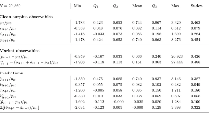
Table 1: Estimation sample summary statistics
N= 29,569 Min Q1 Q2 Mean Q3 Max St.dev.
Clean surplus observables
yit/pit -1.783 0.423 0.653 0.744 0.967 3.320 0.463
xit+1/pit -0.358 0.048 0.076 0.082 0.114 0.512 0.079
dit+1/pit -1.418 -0.033 0.073 0.085 0.198 1.699 0.284
yit+1/pit -1.478 0.424 0.653 0.740 0.963 3.276 0.454
Market observables
(pit+1−pit)/pit -0.959 -0.167 0.033 0.066 0.240 26.923 0.426
r∗
it+1= (pit+1+dit+1−pit)/pit -1.908 -0.118 0.113 0.151 0.363 27.444 0.488
Predictions
ˆ
yit+1/pit -1.350 0.475 0.685 0.740 0.937 3.146 0.387
ˆ
xit+1/pit -0.357 0.055 0.075 0.082 0.102 0.482 0.049
ˆ
dit+1/pit -1.200 -0.005 0.058 0.085 0.150 1.711 0.180
ˆ
xait+1/pit -0.330 0.010 0.033 0.038 0.059 0.697 0.058
( ˆpit+1−pit)/pit -1.602 -0.112 -0.000 -0.028 0.080 1.284 0.190
∆[( ˆpit+1−yˆit+1)/pit] -2.634 -0.123 0.005 -0.000 0.129 3.398 0.322
Note: The statistics for observables and predictions are summarised for the total pooled sample of 29,569 observa-tions. The clean surplus relation is reflected in the arithmetic means: 0.744 + 0.082 - 0.085 = 0.740. The predictions are obtained as per equations10. Table3reports descriptive statistics for the firm-specific parameter estimates, sample sizes and degree of explanatory power associate with these predictions.
Table 1 gives a summary of key statistics over the entire estimation sample, for the observable clean
surplus components, market capital gain and market rate of return, as well for their corresponding
predictions. Table 2 reports the rank correlations for observables, between all reported clean surplus
variables and the realized market rate of return. The table in the Appendix gives the firm-specific
[image:12.595.96.501.538.672.2]samples.
Table 2: Rank correlations for observables
Spearman’sρ
N= 29,569 yit xit+1 dit+1 yit+1 rit+1∗
yit 1 0.4376 0.3869 0.8350 0.3217
xit+1 0.3130 1 0.1392 0.5207 0.3448
Kendall’sτ dit+1 0.2729 0.0996 1 -0.0838 0.4788
yit+1 0.6580 0.3815 -0.0541 1 0.1419
r∗it+1 0.2206 0.2418 0.3419 0.0985 1
Note: All variables are scaled by pit. The rank correlations are reported for the pooled total estimation
5
Analysis
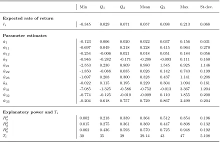
Table3 provides a summarized report of key statistics for the estimated parameters from equations10a
-10c, the coefficients of determination and firm-specific sample sizes. For the expected rate of return, ˆri,
85.44% of firms are recovered with quite reasonable estimates within the range of 0 to the maximum of
0.2134. The remaining 14.56% of firm-specific ˆri are recovered with a negative sign. The mean estimate
is 0.0573 and the median is 0.0707. Past studies have chosen not to report on negative estimates of the
expected rate of return, as it contradicts the intuition in economic theory that firms would not plan ahead
to reduce their market value. As a result, the convention in published work to date is to use reduced
datasets that are consistent with this intuition, particularly by excluding from the estimation sample
any firm-year observation for which the forecast is negative, which would generate a negative estimated
expected return. However, we do not place such restrictions on the explanatory variables, and report
both positive and negative ˆri, which gives a more realistic reflection of realized returns, acknowledging
at the same time the underlying complexity of the empirical study. Nevertheless, the advantage is that
long-run estimates of the rate of return are retrieved from uninterrupted firm-year series, whereas much
research in this area cannot draw generalised conclusions regarding the longer term given that specific
[image:13.595.78.519.373.657.2]firm-years are discarded from estimation when convenient, resulting in incomplete time series.
Table 3: Summary statistics for the 769 firm-specific estimates
Min Q1 Q2 Mean Q3 Max St.dev.
Expected rate of return
ˆ
ri -0.345 0.029 0.071 0.057 0.098 0.213 0.068
Parameter estimates
ˆ
α1 -0.123 0.006 0.020 0.022 0.037 0.156 0.031
ˆ
w11 -0.697 0.049 0.218 0.228 0.415 0.964 0.270
ˆ
w12 -0.254 -0.006 0.021 0.018 0.051 0.184 0.056
ˆ
α2 -0.946 -0.282 -0.171 -0.208 -0.093 0.111 0.160
ˆ
w21 -2.553 0.230 0.809 0.980 1.545 6.925 1.146
ˆ
w22 -1.850 -0.088 0.035 0.026 0.142 0.743 0.199
ˆ
w23 -1.697 0.208 0.300 0.328 0.437 1.141 0.208
ˆ
α3 -0.022 0.115 0.195 0.229 0.304 1.094 0.161
ˆ
w31 -7.085 -1.325 -0.586 -0.752 -0.013 3.367 1.204
ˆ
w32 -0.774 -0.125 -0.010 -0.009 0.110 1.855 0.200
ˆ
w33 -0.204 0.618 0.757 0.729 0.867 2.499 0.204
Explanatory power andTi
R2
x 0.002 0.218 0.339 0.364 0.512 0.854 0.196
R2
d 0.015 0.275 0.361 0.369 0.447 0.808 0.132
R2y 0.062 0.436 0.593 0.570 0.725 0.948 0.192
Ti 30 35 39 39.14 43 47 5.108
Note: The statistics for parameter estimates and explanaotry power reflect frequency-weighted summaries over firm-specific estimation samples. The realised rate of returnr∗it+1is from equation17. The expected rate of return
ˆ
riand the ˆωparameters are estimated as per equations10.R2x,R2dandR
2
dare the associatedR-squares. It holds
thatα3=α1−α2,w31=w11−w21,w32=w12−w22andw33= 1 +r−w23.Tiis the firm-specific sample size.
The Appendix reports a more detailed table of the 769 firm-specific estimates for the ERR, ˆri, with
the respective sample sizesTi and theR-squares. The explanatory power for the firm-specific regressions
givenTi>30 is reasonably high.6 The Appendix table also reports the firm-specific median value of the
Hou, van Dijk, and Zhang (2012) composite measure of the implied cost of capital (ICC).7 By means
of comparison, the median of the ratio of our ˆri over the Hou, van Dijk, and Zhang (2012) median
composite ICC measure is 0.9593 and the mean of this ratio is 1.0914, hence suggesting relatively close
average estimates to the composite ICC, but not necessarily on a firm-by-firm basis.
Evaluating rˆi against its realisations
The estimated ERR, ˆri, with its predicted components from equation14are evaluated against its
respec-tive realisations:
r∗it+1=dit+1
pit
+pit+1−pit
pit
=xit+1
pit
−yit+1−yit
pit
+pit+1−pit
pit
, (17)
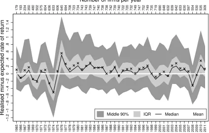
Figure1 shows the year-specific difference between the realized rate or returnr∗
it+1 and the expected
rate of return, ˆri, in terms of middle 90% (the 95th minus the 5th percentile), the interquartile range
(IQR), the median and the arithmetic mean estimates. During recessionary periods, ˆri is much higher
than r∗it+1 and during expansionary periods the opposite holds. This suggests a steeper impact on the
market’s realised rate of return when taking in bad news by comparison to good news, generally consistent
with theKahneman and Tversky(1979) Prospect Theory.8
To test the effectiveness of our accounting data-driven method to estimating a representative rate of
expected return, we test whether the realized rate of returns,rit+1∗ , revert to their long-run average, ˆri,
as estimated by the linear information system of equations 10a - 10c. If ˆri is a reasonable estimate of
the long-run rate of the ERR, then the mean-reversion of the realized rate of return to ˆri should be
strong. Returns are stationary over time and mean-reverting, hence a mean-reverting test can be stated
in discrete time as a test for a stationary process (Cochrane 2001). In this respect, we may rewriter∗it+1
as a weighted average of its past value and its expectation:
r∗it+1= (1−φi)rit∗ +φiˆri+it+1 (18)
whereit+1is a random Normal shock. The null hypothesis for mean-reversion is stated asH0:−φi=
−1. Given that ˆri is a firm-specific estimate, the regression test specified in equation 18 amounts to a regression on a slope coefficient with inverted sign. For the level of significance α= 0.01, we fail to
reject the null for 580 out of 769 firm-specific time series. Hence, the mean-reversion test suggests that
for 75.42% of the firms withTi >30 during 1964-2011, the future realized rate of return,rit+1∗ , reverts
6A more complete report, including firm-specific estimates for theω parameters from equations10a-10c, is available
upon request.
7This composite measure is the average ICC as estimated byEaston (2004), Gordon and Gordon(2002), Claus and Thomas(2001),Gebhardt, Lee, and Swaminathan(2001), andOhlson and Juettner-Nauroth(2005). With thanks to Kewei Hou for providing the firm-specific estimates fromHou, van Dijk, and Zhang(2012).
8Using the National Bureau of Economic Research definition of business cycle, the list of US recessions during the
Figure 1: Difference between realized and expected rate of return per year
−1.2
−1
−.8
−.6
−.4
−.2
0
.2
.4
.6
.8
1
1.2
1.4
Realised minus expected rate of return
179 193 234 350 480 502 575 604 636 633 606 645 694 708 723 734 743 743 739 747 740 738 738 742 739 740 722 720 732 749 747 752 749 735 719 690 648 632 639 642 633 630 597 554 530 535 309
Number of firms per year
1965 1966 1967 1968 1969 1970 1971 1972 1973 1974 1975 1976 1977 1978 1979 1980 1981 1982 1983 1984 1985 1986 1987 1988 1989 1990 1991 1992 1993 1994 1995 1996 1997 1998 1999 2000 2001 2002 2003 2004 2005 2006 2007 2008 2009 2010 2011
Middle 90% IQR Median Mean
They-axis gives the year-specific differences between the realized rate of returnr∗it+1from equation17and the expected rate of return ˆri. The differences are shown for the middle middle 90% (the 95thminus 5thpercentile), the interquartile
range (IQR), the median and the arithmetic mean estimates. The superimposed white line indicatesr∗
it+1−ˆri= 0. The
bottomx-axis shows the timeline where the topx-axis reports the year-specific sample size (number of firms per year).
to ˆri on average, and that past changes in price do not help predict future returns in the market. The
Appendix reports the firm-specific estimates for ˆφi.9
Evaluating the components of rˆi
To evaluate the relation between the components of the predicted ERR, ˆri (equation 14), against the
respective realisations as well against the realized rate of return, r∗
it+1 (equation 17), we apply the
exploratory method of portfolio smoothing. The total sample of N = 29,569 observations is grouped
into 296 portfolios each containing 99 or 100 observations summing up to the total. For everyy=f(x)
relation that is graphed, we first calculate the median expectation for the x-axis variable per portfolio,
and on the basis of this median we calculate the three quartiles of the y-axis variable.10 The resulting
graph is a smoothed summary of central tendency for consecutive localities of the bivariate distribution.
In addition, we plot the non-parametric estimates for cubic splines with five knots in order to assess the
9Standard error estimates are corrected via the Eicker-Huber-White ‘sandwich’ robust estimator and are available upon
request.
10Portfolio smoothing summarizes consecutive localities of the bivariate distribution and therefore eliminates noise hence
revealing hidden patterns in the data. For the origins of this method, sometimes also referred to asquantile smoothing, see
nature of relationship without having to impose a rigid functional form.11 This exploratory approach
is applied in a consistent manner for Figures 4 to 7 for the predicted components of ˆri, that is for the
predicted capital gain, net earnings, net dividend, change in book value of equity, abnormal earnings and
change in unrecorded goodwill, respectively.
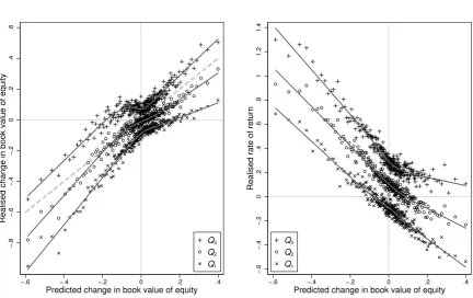
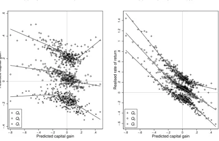
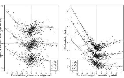
Figures2-5 evaluate the various components of ˆri in terms of (i) their impact on the accuracy of ˆrias
a predictor of one-year ahead realized stock returns (left-hand side plots), and (ii) their own ability to
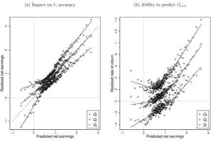
[image:16.595.81.518.209.500.2]predict future realized stock returns ˆrit+1∗ (right-hand side plots).
Figure 2: Predicted net earnings
(a) Impact on ˆriaccuracy
−.1
0
.1
.2
.3
Realised net earnings
−.1 0 .1 .2 .3
Predicted net earnings
Q3
Q2
Q1
(b) Ability to predict ˆr∗it+1
−.4
−.2
0
.2
.4
.6
.8
1
1.2
1.4
Realised rate of return
−.1 0 .1 .2 .3
Predicted net earnings
Q3
Q2
Q1
They-axis of the left-hand side graph gives the quartiles of realized net earningsxit+1/pit. They-axis of the right-hand
side graph gives the quartiles of the realized rate of returnr∗it+1. The quartiles of bothy-axes variables are calculated on the basis of the portfolio-specific median of thex-axis variable of the predicted net earnings, ˆxit+1/pit. There are
296 portfolios each with 99 or 100 observations summing to the total ofN= 29,569. To assist visual representation, the graph suppresses the display of the two most extreme portfolios, those with the minimum and maximum ˆxit+1/pit. The
overlaid lines reflect estimation of cubic splines with five knots. The diagonal dashed line references the 45o degree line
wherey=x.
Focusing first on the impact of each component of ˆri given by equation14 on the accuracy of ˆri as a
predictor of one-year ahead realized stock returns, Figures2aand3aconfirm a strong positive association
between predicted earnings and predicted change in book value and their corresponding component of
realized stock returns. Figure 4a, on the other hand, indicates that, while there is broad agreement
between the predicted and the realized capital gain for the typical portfolio i.e. high bivariate density
concentration around zero, there is a negative relation between predicted and realized capital gains for
the median realized capital gain observed in each portfolio. In particular, for portfolios with significantly
negative predicted capital gains, the median realized capital gain turns out to be significantly positive.
These results suggest that the substantial deviations of ˆrit+1∗ from ˆri documented in Figure 1 may be
principally explained by the capital gain component of ˆri as opposed to the accounting components.
Figure 3: Predicted change in book value of equity
(a) Impact on ˆriaccuracy
−.8
−.6
−.4
−.2
0
.2
.4
.6
Realised change in book value of equity
−.6 −.4 −.2 0 .2 .4
Predicted change in book value of equity Q3
Q2
Q1
(b) Ability to predict ˆr∗it+1
−.6
−.4
−.2
0
.2
.4
.6
.8
1
1.2
1.4
Realised rate of return
−.6 −.4 −.2 0 .2 .4
Predicted change in book value of equity Q3
Q2
Q1
They-axis of the left-hand side graph gives the quartiles of realized change in book value of equity (yit+1−yit)/pit. The
y-axis of the right-hand side graph gives the quartiles of the realized rate of return r∗
it+1. The quartiles of both y-axes
variables are calculated on the basis of the portfolio-specific median of thex-axis variable of the predicted change in book value of equity, (ˆyit+1−yit)/pit. There are 296 portfolios each with 99 or 100 observations summing to the total of
N= 29,569. To assist visual representation, the graph suppresses the display of the two most extreme portfolios, those with the minimum and maximum (ˆyit+1−yit)/pit. The overlaid solid lines reflect estimation of cubic splines with five
knots. The diagonal dashed line references the 45o degree line wherey=x.
Given that ˆri is an average long-run measure of the ERR, it is not surprising that it is a noisy
predictor of short-run realized stock returns, ˆr∗it+1. Specifically, consistent with perspectives of Penman
(2016) andCallen(2016) in this issue, if there are short-run variations in the ERR and these are positively
(negatively) associated with the net earnings (change in book value of equity) components of ˆri, this will
both weaken the association of ˆriwith realized stock returns and potentially create a negative association
between the capital gain component of ˆri and realized stock returns. Evidence in Figures 2b and 3b
strongly suggest that net earnings (change in book value of equity) scaled by opening market value of
equity are positively (negatively) related to future stock returns and this in turn results in the apparently
perverse result in Figure 4bthat the predicted capital gain component of ˆri strongly negatively related
to future stock returns. The latter is simply due to the indirect estimation of the predicted capital gain
component as ˆri minus the predicted net earnings component plus the predicted change in book value
of equity component i.e. if the net earnings component is positively related to the short-run ERR (and
to one-year ahead realized stock returns) and if the book value of equity component is negatively related
to the short-run ERR (and the one year ahead realized stock returns), then it follows that the predicted
capital gain component will be negatively related to short-run ERR (and one year ahead stock returns)
Figure 4: Predicted capital gain
(a) Impact on ˆriaccuracy
−.4
−.2
0
.2
.4
.6
Realised capital gain
−.8 −.6 −.4 −.2 0 .2 .4
Predicted capital gain Q3
Q2
Q1
(b) Ability to predict ˆr∗it+1
−.6
−.4
−.2
0
.2
.4
.6
.8
1
1.2
1.4
Realised rate of return
−.8 −.6 −.4 −.2 0 .2 .4
Predicted capital gain Q3
Q2
Q1
They-axis of the left-hand side graph gives the quartiles of the realized capital gain (pit+1−pit)/pit. They-axis of the
right-hand side graph gives the quartiles of the realized rate of return r∗
it+1. The quartiles of both y-axes variables
are calculated on the basis of the portfolio-specific median of thex-axis variable of the predicted capital gain, ( ˆpit+1− pit)/pit. There are 296 portfolios each with 99 or 100 observations summing to the total of N = 29,569. To assist
visual representation, the graph suppresses the display of the two most extreme portfolios, those with the minimum and maximum ( ˆpit+1−pit)/pit. The overlaid lines reflect estimation of cubic splines with five knots.
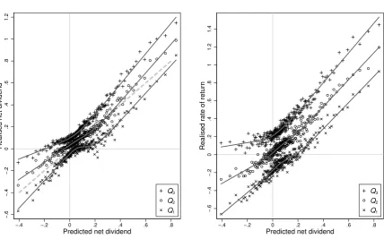
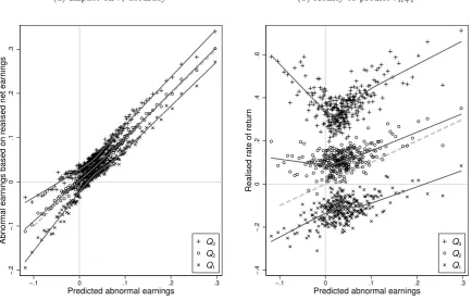
Further results reported in Figures5-7support the view that the time-varying accounting components
of ˆri capture the short-run variation of ERR around its long-run expected rate. First, Figure5indicates
that when predicted earnings and predicted change in book value of equity are combined to form
pre-dicted net dividends, this composite accounting component is strongly associated with future realized net
dividends and, more importantly, strongly related to the realized stock returns. Second, Figure6provides
further evidence on the role of predicted abnormal earnings as a predictor of future stock returns which
is broadly consistent with, but somewhat weaker than, the results reported for predicted net earnings.
Finally, Figure7shows that when the last two components of ˆri in equation14are combined to form
predicted change in unrecorded goodwill, this composite variable broadly shares the negative association
with its own future realisation as for predicted capital gains (however there are some evidence of a
positive association for the majority of portfolios with small positive predicted changes in goodwill as
shown in Figure7a), but is less strongly negatively associated with future stock returns than was the case
for predicted capital gains as shown in Figure 7b. Interestingly, the latter implies that if our long-run
ERR estimate is simply dichotomised into a predicted earnings component and an unrecorded goodwill
component, then comparison of Figures2band7bprovide strong evidence that the earnings component
has a stronger and more consistently positive association with short-run variation in the ERR reflected
Figure 5: Predicted net dividend
(a) Impact on ˆriaccuracy
−.6
−.4
−.2
0
.2
.4
.6
.8
1
1.2
Realised net dividend
−.4 −.2 0 .2 .4 .6 .8
Predicted net dividend
Q3
Q2
Q1
(b) Ability to predict ˆr∗it+1
−.6
−.4
−.2
0
.2
.4
.6
.8
1
1.2
1.4
Realised rate of return
−.4 −.2 0 .2 .4 .6 .8
Predicted net dividend
Q3
Q2
Q1
They-axis of the left-hand side graph gives the quartiles of realized net dividenddit+1/pit. They-axis of the right-hand
side graph gives the quartiles of the realized rate of returnr∗
it+1. The quartiles of bothy-axes variables are calculated on
the basis of the portfolio-specific median of thex-axis variable of the predicted net dividend, ˆdit+1/pit. There are 296
portfolios each with 99 or 100 observations summing to the total ofN= 29,569. To assist visual representation, the graph suppresses the display of the two most extreme portfolios, those with the minimum and maximum ˆdit+1/pit. The overlaid
solid lines reflect estimation of cubic splines with five knots. The diagonal dashed line references the 45odegree line where
y=x.
In summary, our empirical analysis has provided firm-specific estimates of the long-run expected return
on equity, based on the constrained estimation of a system of accounting-based forecast models, which
are related to firm-specific implied cost of capital estimates generated in prior research. Our analysis
indicates that realized stock returns on average revert to the estimated ERR but that, consistent with
prior research by Easton and Monahan(2005) on the implied cost of capital, there is no evidence that
our estimate of ERR predicts one-year ahead realized stock returns. Further analysis, however, indicates
that the time-varying accounting components of our firm-specific ERR estimates are strongly related at
a portfolio level to future realized stock returns. This is consistent with time variation in ERRs around a
long-run average where predicted net earnings and predicted net dividends scaled by equity value provide
useful additional information on short-run variations in the ERR.
6
Conclusions
The method for estimating the expected rate of return that is described in this paper adapts the linear
information model that is based on abnormal earnings to a reported earnings basis, and then imposes
the clean surplus parameter constraints identified in Clubb (2013). The resulting equation system is
rank deficient and, following the methods described byChristodoulou and McLeay(2014), we identify its
Figure 6: Predicted abnormal earnings
(a) Impact on ˆriaccuracy
−.2
−.1
0
.1
.2
.3
Abnormal earnings based on realised net earnings
−.1 0 .1 .2 .3
Predicted abnormal earnings
Q3
Q2
Q1
(b) Ability to predict ˆr∗it+1
−.4
−.2
0
.2
.4
.6
Realised rate of return
−.1 0 .1 .2 .3
Predicted abnormal earnings
Q3
Q2
Q1
They-axis of the left-hand side graph gives the quartiles of abnormal earnings based on realized net earningsxa
it+1/pit=
xit+1/pit−ri×yit/pit. They-axis of the right-hand side graph gives the quartiles of the realized rate of returnr∗it+1.
The quartiles of bothy-axes variables are calculated on the basis of the portfolio-specific median of thex-axis variable of the predicted abnormal earnings, ˆxa
it+1/pit, from equation13. There are 296 portfolios each with 99 or 100 observations
summing to the total ofN = 29,569. To assist visual representation, the graph suppresses the display of the two most extreme portfolios, those with the minimum and maximum ˆxa
it+1/pit. The overlaid lines reflect estimation of cubic splines
with five knots. The diagonal dashed line references the 45odegree line wherey=x.
accounting identity. In contrast to previous research on the ‘implied cost of capital’, the long-run ERR
estimates reported in this paper are based purely on the firm’s accounting information dynamics and
without reference to its stock price or market analysts’ forecasts. In other words, these estimates are
based on evidence regarding the persistence of each firm’s accounting performance in its product markets,
as opposed to assessments by the capital market of the firm’s future performance. Interestingly, the
average of our firm-specific ERRs is similar to the average based on prior research on the implied cost of
capital, although -not surprisingly- there are differences at the firm level.
In addition to providing accounting-based estimates of firm-specific ERRs, we investigate the
rela-tionship between our ERR estimates and future realised one-year ahead stock returns in line with prior
research on the implied cost of capital, and make use of our accounting-based approach to analyse the
usefulness of ERR components with respect to predictions of earnings, dividends and book value.
Con-sistent with previous research on the market reaction to released accounting information, there is no
simple linear relation between our ERR estimates and realised stock returns, but we do find evidence
that average realised stock returns are related to average ERR over the full sample period 1961-2011.
Using a portfolio smoothing method, evidence suggests that the articulated components of the estimated
ERR (i.e. articulated such that predicted net earnings, less predicted change in book value of equity is
equal to predicted net dividends, and where each is scaled by opening market value of equity) are strongly
positively related to one year ahead realised stock returns, but that predicted capital gains and predicted
Figure 7: Predicted change in unrecorded goodwill
(a) Impact on ˆriaccuracy
−.4
−.2
0
.2
.4
.6
Realised change in unrecorded goodwill
−1 −.8 −.6 −.4 −.2 0 .2 .4 .6 .8 1
Predicted change in unrecorded goodwill Q3
Q2
Q1
(b) Ability to predict ˆr∗it+1
−.2
0
.2
.4
.6
.8
1
1.2
Realised rate of return
−1 −.8 −.6 −.4 −.2 0 .2 .4 .6 .8 1
Predicted change in unrecorded goodwill Q3
Q2
Q1
They-axis of the left-hand side graph gives the quartiles of realized change in unrecorded goodwill ∆[(pit+1−yit+1)/pit].
The y-axis of the right-hand side graph gives the quartiles of the realized rate of return r∗
it+1. The quartiles of both y-axes variables are calculated on the basis of the portfolio-specific median of thex-axis variable of the predicted change in unrecorded goodwill, ∆[( ˆpit+1−yˆit+1)/pit]. There are 296 portfolios each with 99 or 100 observations summing to the
total ofN= 29,569. To assist visual representation, the graph suppresses the display of the two most extreme portfolios, those with the minimum and maximum ∆[( ˆpit+1−yˆit+1)/pit]. The overlaid solid lines reflect estimation of cubic splines
with five knots. The diagonal dashed line references the 45odegree line wherey=x.
realised stock returns. We interpret this as consistent with short-term variation from the long-run ERR
(presumably related to changes in risk), and also as evidence of the usefulness of accounting predictions
in forecasting short-run stock returns.
We conclude that this study provides a promising new approach to the estimation of a long-run
expected rate of return, which highlights the important role of accounting fundamentals in the assessment
of firm risk. While our approach avoids the use of stock prices to reverse-engineer expected rates of return,
the underlying role of abnormal earnings dynamics clearly emphasises the importance of the capital
market’s return expectations in influencing competition between firms and hence firm performance. We
hope that future research might further explore the relationship between, and relative performance of,
Appendix: Firm-specific estimates for companies with
T
i≥
30
Company name Ti ˆri ICC φi R2x R2d R2y Company name Ti ˆri ICC φi R2x R2d R2y
3M 46 0.084 0.051 -1.10* 0.47 0.31 0.79 AAR 41 0.065 -0.74* 0.34 0.27 0.39
AMP 34 -0.060 0.049 -0.81* 0.42 0.33 0.60 AT&T 39 0.082 0.026 -1.06* 0.18 0.32 0.64
AZZ 33 0.078 0.125 -0.83* 0.39 0.47 0.17 Abbott Laboratories 47 0.092 0.050 -1.28* 0.26 0.42 0.83
Abm Industries 43 0.079 0.096 -0.78* 0.43 0.29 0.45 Aceto 37 0.111 0.121 -0.80* 0.38 0.55 0.28
Acme United 37 -0.069 0.159 -0.58 0.40 0.32 0.22 Adams Resources 33 -0.037 0.127 -0.80* 0.25 0.35 0.67
Adv. Micro Devices 36 0.077 0.052 -0.93* 0.04 0.49 0.34 Aeroquip-Vickers 30 0.015 0.088 -0.85* 0.29 0.13 0.64
Agilysys 34 0.084 0.115 -0.90* 0.12 0.65 0.34 Agl Resources 44 0.112 0.102 -0.58 0.66 0.24 0.78
Air Products & Chem. 47 0.020 0.062 -0.99* 0.17 0.23 0.48 Airborne 32 -0.030 0.088 -0.77* 0.15 0.53 0.35
Alaska Air Group 38 0.009 0.100 -0.75* 0.45 0.54 0.57 Alberto-Culver 43 0.042 0.093 -0.56 0.38 0.22 0.78
Albertson’s 38 0.079 0.072 -0.96* 0.70 0.40 0.64 Alcan 42 0.133 0.075 -0.93* 0.48 0.27 0.48
Alcoa 47 0.032 -1.04* 0.25 0.29 0.61 Alexander & Baldwin 39 0.098 0.086 -0.94* 0.54 0.39 0.74
Alico 47 0.029 0.075 -0.69 0.34 0.41 0.74 Allegheny Energy 45 0.096 0.095 -0.76* 0.61 0.34 0.67
Allegheny Tech. 43 0.093 0.121 -0.73 0.40 0.36 0.30 Allen Telecom 31 0.090 0.081 -0.92* 0.24 0.49 0.44
Allete 47 0.112 0.096 -0.79* 0.61 0.44 0.77 Alliant Energy 43 0.075 0.096 -0.92* 0.20 0.40 0.19
Alltel 38 0.093 0.088 -0.75* 0.63 0.22 0.74 Altria Group 47 0.048 0.047 -0.99* 0.27 0.39 0.87
Ameren 47 0.096 -0.59 0.72 0.38 0.75 American Elec. Power 46 0.039 0.092 -0.81* 0.58 0.30 0.51
American Greetings 44 0.087 0.077 -0.50 0.18 0.37 0.71 American Science Eng. 40 0.125 0.065 -0.78* 0.45 0.33 0.63
American Stores 30 0.114 0.088 -0.93* 0.46 0.49 0.35 American Water Works 31 0.088 0.112 -0.63* 0.82 0.25 0.81
Ameron Int’l 40 0.077 0.118 -0.74* 0.34 0.32 0.59 Ametek 43 0.063 0.071 -0.81* 0.41 0.34 0.57
Amoco 30 0.071 0.044 -0.77* 0.38 0.32 0.41 Ampco-Pittsburgh 36 0.029 0.112 -0.67 0.25 0.25 0.48
Amrep 31 0.066 0.073 -0.68* 0.38 0.38 0.52 Analog Devices 40 0.042 0.048 -0.72 0.50 0.31 0.52
Analogic 34 0.055 0.055 -0.71 0.68 0.69 0.64 Angelica 42 0.082 0.092 -0.54 0.54 0.26 0.59
Anheuser-Busch Cos 41 0.125 0.063 -0.74* 0.76 0.36 0.86 Anixter Intl 33 0.129 0.049 -0.81* 0.32 0.11 0.60
Apache 43 0.134 0.076 -0.80* 0.50 0.39 0.50 Apogee Enterprises 35 0.091 0.093 -0.63* 0.43 0.45 0.50
Applied Biosystems 40 0.041 0.047 -1.09* 0.11 0.38 0.54 Applied Industrial Tech 44 -0.053 0.080 -0.66 0.26 0.25 0.41
Applied Materials 33 0.111 0.048 -0.97* 0.32 0.23 0.33 Aqua America 39 -0.116 0.095 -0.62* 0.58 0.34 0.32
Aquila 36 0.089 0.114 -0.77* 0.53 0.37 0.51 Archer-Daniels Mid. 45 0.014 0.067 -0.82* 0.25 0.42 0.48
Arkansas Best 31 0.170 0.099 -0.86* 0.26 0.68 0.45 Arrow Electronics 32 0.122 0.094 -1.02* 0.16 0.52 0.23
Arts Way Mfg 32 0.110 0.150 -0.90* 0.11 0.69 0.26 Arvin Industries 31 0.116 0.099 -0.70 0.45 0.38 0.55
Ashland 44 0.107 0.096 -0.74* 0.14 0.37 0.39 Astronics 30 0.114 0.179 -0.62* 0.20 0.69 0.61
Atlantic Energy 33 0.062 0.110 -0.61 0.64 0.31 0.71 Atlantic Richfield 33 -0.008 0.054 -0.60 0.31 0.32 0.73
Atrion 40 0.060 0.151 -0.65 0.07 0.23 0.62 Atwood Oceanics 34 0.049 0.069 -0.71* 0.26 0.15 0.54
Automatic Data Proces. 43 -0.132 0.044 -0.90* 0.46 0.38 0.44 Avery Dennison 43 0.101 0.056 -0.89* 0.23 0.21 0.83
Avista 46 0.061 -0.81* 0.28 0.41 0.44 Avnet 43 0.094 0.073 -0.75* 0.36 0.41 0.36
Avon Products 44 -0.005 0.056 -1.07* 0.01 0.08 0.81 Axsys Technologies 32 0.116 0.082 -0.83* 0.30 0.40 0.39
BALL 37 0.091 0.076 -0.74* 0.50 0.50 0.87 BEAM 46 0.116 0.080 -0.75 0.44 0.34 0.76
BP 40 0.107 0.256 -0.65 0.26 0.39 0.67 Badger Meter 37 0.057 0.173 -0.79* 0.43 0.17 0.79
Bairnco 31 0.135 0.130 -0.76* 0.19 0.59 0.48 Baker (Michael) 39 -0.006 0.137 -0.68 0.13 0.27 0.50
Baker Hughes 42 -0.077 0.051 -0.71 0.05 0.41 0.18 Baldor Electric 31 0.029 0.061 -0.97* 0.34 0.30 0.47
Bandag 36 0.022 0.074 -0.73* 0.42 0.20 0.68 Bard (C.R.) 44 0.100 0.058 -0.89* 0.49 0.32 0.72
Barnes Group 44 0.046 0.091 -1.05* 0.20 0.32 0.54 Barnwell Industries 42 -0.029 0.146 -0.83* 0.11 0.12 0.73
Barry (R G) 35 0.020 0.107 -0.64* 0.03 0.35 0.53 Bassett Furniture 37 -0.033 0.083 -0.54 0.52 0.25 0.45
Bat-British Amer Tob. 31 0.133 1.306 -0.86* 0.85 0.39 0.85 Bausch & Lomb 42 0.092 0.060 -1.13* 0.21 0.54 0.38
Baxter Int’l 47 0.066 0.047 -0.94* 0.28 0.33 0.58 Beckman Coulter 37 -0.002 0.046 -0.97* 0.01 0.28 0.37
Becton Dickinson 43 0.063 0.057 -0.99* 0.21 0.31 0.69 Bemisinc 43 0.064 0.085 -0.97* 0.40 0.14 0.80
Bestfoods 33 0.112 0.071 -1.03* 0.71 0.20 0.86 Biglari Hldg 41 -0.060 0.119 -0.99* 0.36 0.59 0.50
Bio-Rad Laboratories 35 0.082 0.106 -0.85* 0.14 0.56 0.30 Black Hills 43 0.069 0.103 -0.88* 0.63 0.35 0.75
Black & Decker 41 -0.077 0.057 -0.70 0.06 0.01 0.51 Blair 38 0.008 0.092 -0.89* 0.03 0.34 0.68
Block H & R 42 0.130 0.061 -0.92* 0.44 0.54 0.76 Blount Intl 33 0.075 0.122 -0.82* 0.28 0.20 0.69
Bob Evans Farms 38 -0.090 0.064 -0.66 0.35 0.43 0.39 Boeing 43 0.027 0.069 -0.74* 0.67 0.62 0.82
Bowl America 35 0.061 0.227 -0.50 0.83 0.42 0.70 Bowneinc 38 0.109 0.089 -0.83* 0.56 0.70 0.50
Breeze-Eastern 33 0.056 0.132 -0.49 0.17 0.28 0.71 Bridgford Foods 39 0.089 0.203 -0.57 0.36 0.45 0.78
Briggs & Stratton 43 -0.044 0.069 -0.77* 0.15 0.30 0.54 Bristol-Myers Squibb 47 0.104 0.049 -1.09* 0.28 0.24 0.80
Bristow Group 31 0.071 0.092 -0.80* 0.53 0.52 0.24 Brown Shoeinc 43 0.148 0.082 -0.58 0.47 0.43 0.42
Brown-Forman 46 0.093 0.098 -0.77* 0.64 0.38 0.78 Brunswick 41 0.094 0.072 -0.79* 0.53 0.20 0.67
Butler Mfg 33 -0.010 0.110 -0.54 0.15 0.35 0.29 CBS 35 0.035 0.075 -0.95* 0.10 0.55 0.17
CBS 30 -0.070 0.072 -0.58 0.17 0.19 0.46 CDI 39 -0.004 0.088 -0.54 0.43 0.30 0.54
COHU 40 0.087 0.166 -0.72* 0.38 0.48 0.54 CSX 37 0.024 0.081 -0.97* 0.14 0.11 0.66
CTS 43 0.079 0.083 -0.68 0.27 0.27 0.45 Cabot 42 0.086 0.075 -0.90* 0.27 0.67 0.80
Caci Intl 30 0.076 0.054 -0.86* 0.22 0.46 0.46 Campbell Soup 43 0.054 0.060 -1.00* 0.52 0.12 0.92
Canon 30 0.006 0.948 -0.97* 0.15 0.43 0.30 Capital Cities/Abc 30 0.056 0.064 -0.90* 0.10 0.43 0.35
Carpenter Technology 43 0.113 0.085 -0.59 0.43 0.29 0.47 Carter-Wallace 32 0.046 0.081 -0.59* 0.35 0.29 0.78
Cascade 38 0.133 0.135 -0.75* 0.51 0.36 0.74 Cascade Natural Gas 39 0.097 0.141 -0.91* 0.38 0.58 0.76
Castle (A M) 41 0.097 0.133 -0.58 0.46 0.35 0.81 Caterpillar 43 -0.087 0.060 -0.69 0.23 0.23 0.80
Cbs-Old 35 0.104 0.082 -0.80* 0.43 0.27 0.59 Centerior Energy 31 0.074 -0.97* 0.30 0.29 0.65
Centerpoint Energy 45 0.099 0.092 -0.79* 0.38 0.31 0.79 Centex 36 0.058 0.080 -0.76* 0.25 0.47 0.22
Central Vermont Pub. 43 0.089 0.132 -0.61 0.24 0.40 0.57 Central & South West 35 0.107 0.095 -0.54 0.84 0.43 0.89
Centurylink 35 0.094 0.108 -0.87* 0.64 0.31 0.71 Ch Energy Group 47 0.111 0.114 -0.77* 0.26 0.38 0.66
Champion Int’l 34 0.013 0.081 -0.81* 0.31 0.25 0.48 Charming Shoppes 33 0.079 0.066 -0.73* 0.26 0.73 0.66
Chase 33 -0.002 0.130 -0.61* 0.15 0.49 0.20 Chattem 34 0.048 0.084 -0.81* 0.12 0.22 0.65
Chemed 38 -0.176 0.070 -0.51 0.12 0.45 0.21 Chemtura 42 0.077 0.099 -0.94* 0.31 0.20 0.71
Chesapeake Utilities 31 0.137 0.164 -0.79* 0.85 0.59 0.74 Chevron 47 0.047 0.041 -0.69 0.42 0.18 0.70
Chicago Rivet 41 -0.081 0.240 -0.64* 0.32 0.35 0.48 Church & Dwight 32 0.120 0.066 -1.13* 0.73 0.37 0.85
Cincinnati Bell 39 0.068 0.090 -0.62* 0.49 0.41 0.95 Cipsco 32 0.087 -0.66 0.57 0.32 0.69
Clarcor 41 0.064 0.074 -0.94* 0.54 0.41 0.48 Cleco 41 0.120 0.089 -0.81* 0.44 0.47 0.63
Cliffs Natural Res. 43 -0.345 0.090 -0.58 0.49 0.37 0.45 Clorox Co/De 41 0.087 0.062 -0.72* 0.56 0.30 0.78
Cmp Group 35 0.091 0.113 -0.74* 0.30 0.29 0.52 Cms Energy 42 0.076 0.103 -0.72* 0.35 0.39 0.71
Coca-Cola 47 0.125 0.042 -1.26 0.58 0.36 0.78 Coca-Cola Btlng Cons 33 0.051 0.075 -0.91* 0.27 0.31 0.85
Coherent 37 0.111 -0.84* 0.27 0.71 0.26 Colgate-Palmolive 47 0.048 0.058 -0.77* 0.25 0.14 0.89
Comcast 35 0.122 0.023 -0.79* 0.36 0.41 0.68 Commercial Metals 41 0.048 0.114 -0.88* 0.41 0.39 0.62
Commonwlth Energy 34 0.095 0.130 -0.63 0.61 0.29 0.51 Commonwlth Tel. 36 0.098 0.152 -1.18* 0.54 0.32 0.81
Computer Sciences 43 0.073 0.069 -0.78* 0.27 0.25 0.58 Comsat -Ser 1 30 0.060 0.075 -0.71* 0.09 0.28 0.51
Con-Way 42 0.089 0.081 -0.70* 0.20 0.28 0.41 Conagra Foods 38 0.117 -0.82* 0.85 0.81 0.84
Conocophillips 44 0.064 0.069 -0.86* 0.06 0.34 0.31 Consolidated Edison 45 0.092 0.106 -0.76* 0.84 0.58 0.88