PAPER • OPEN ACCESS
Current large deviations for partially asymmetric particle systems on a
ring
To cite this article: Paul Chleboun et al 2018 J. Phys. A: Math. Theor. 51 405001
Journal of Physics A: Mathematical and Theoretical
Current large deviations for partially
asymmetric particle systems on a ring
Paul Chleboun1 , Stefan Grosskinsky2
and Andrea Pizzoferrato3,4,5
1 Department of Statistics, University of Oxford, Oxford, United Kingdom 2 Mathematics Institute, University of Warwick, Coventry, United Kingdom 3 Department of Mathematics, Imperial College, London, United Kingdom 4 The Alan Turing Institute, London, United Kingdom
E-mail: [email protected]
Received 24 April 2018, revised 15 August 2018 Accepted for publication 23 August 2018 Published 10 September 2018
Abstract
We study large deviations for the current of one-dimensional stochastic particle systems with periodic boundary conditions. Following a recent approach based on an earlier result by Jensen and Varadhan, we compare several candidates for atypical currents to travelling wave density profiles, which correspond to non-entropic weak solutions of the hyperbolic scaling limit of the process. We generalize previous results to partially asymmetric systems and systems with convex as well as concave current-density relations, including zero-range and inclusion processes. We provide predictions for the large deviation rate function covering the full range of current fluctuations using heuristic arguments, and support them by simulation results using cloning algorithms wherever they are computationally accessible. For partially asymmetric zero-range processes we identify an interesting dynamic phase transition between different strategies for atypical currents, which is of a generic nature and expected to apply to a large class of particle systems on a ring.
Keywords: large deviations, current fluctuations, stochastic lattice gases
(Some figures may appear in colour only in the online journal)
P Chleboun et al
Current large deviations for partially asymmetric particle systems on a ring
Printed in the UK 405001
JPHAC5
© 2018 IOP Publishing Ltd 51
J. Phys. A: Math. Theor.
JPA
1751-8121
10.1088/1751-8121/aadc6e
Paper
40
1
23
Journal of Physics A: Mathematical and Theoretical
2018
Original content from this work may be used under the terms of the Creative Commons Attribution 3.0 licence. Any further distribution of this work must maintain attribution to the author(s) and the title of the work, journal citation and DOI.
5 Author to whom any correspondence should be addressed.
1. Introduction
Large deviations of dynamic observables in bulk-driven lattice gases have been a topic of major recent research interest. As summarized in a recent review [1], most studies focus on the empirical particle current as one of the most important characteristics of nonequilibrium sys-tems in one dimension. To derive the large deviation rate function for additive path functionals such as the current, the associated scaled cumulant generating function can be characterized in terms of the leading eigenvalue of a tilted version of the generator of the process [2]. In many cases an ansatz for the corresponding eigenfunction can be derived and such microscopic methods have been applied successfully to various models: to the asymmetric simple exclu-sion process (ASEP) [3, 4] based on Bethe-ansatz type techniques related to exact solvability, and also in combination with the matrix product ansatz [5], and to zero-range processes (ZRP) [6–8] based on existence of non-homogeneous factorized stationary distributions. The typical scenario for these studies is open boundary conditions, due to its rich behaviour determined by the additional degree of freedom from coupling with particle reservoirs. This paper fills a gap in the literature by addressing the periodic case, where only few results exist so far [9–12]. Dynamic large deviations have also been studied successfully from a macroscopic point of view using more generally applicable techniques, most notably macroscopic fluctuation the-ory (MFT) (see [13] and references therein), which can be understood in terms of empirical flows for Markov chains [14, 15]. The time evolution of the most likely density profile for a given fluctuation of the current is characterized by a variational principle, which can be hard to solve in general, and explicit expressions have only been obtained for some specific models so far [1, 13]. A priori this approach is limited to symmetric or weakly asymmetric bulk dynam-ics, but full asymmetry can often be covered in the limit of a diverging weak field.
In general, macroscopic approaches rely on a hydrodynamic description of the process in terms of a conservation law. For asymmetric models this is a hyperbolic equation with weak solutions that can develop shock discontinuities, and for which additional selection cri-teria are needed to identify a unique (entropic) solution, such as a fixed positive sign for the entropy production (see e.g. [16]). Provided the ‘correct’ thermodynamic entropy functional is used, the negative part of the entropy production provides the large deviation rate function for observing a non-entropic weak solution in the scaling limit [17]. This general idea has been proved rigorously only for the ASEP so far [18, 19]. In [20], this has been applied heuristi-cally to obtain the rate function for lower current deviations for the ASEP, which are realized by phase separated (travelling wave) profiles where two regions of different densities are separated by two shock discontinuities, in agreement with exact microscopic results. In recent work [21] this approach has been shown to apply also for totally asymmetric ZRPs with con-cave current-density relation, where the validity can be limited by a crossover to condensed profiles in certain models constituting a dynamic phase transition. Similar results on dynamic phase transitions can be found in [22, 23] for the periodic total ASEP (TASEP), [24–26] for the periodic weakly asymmetric simple exclusion process (WASEP), [27, 28] for the open WASEP and [29] for open and periodic non-integrable ASEPs.
studied in the context of condensation [37], together with certain variations (see [38]). For this paper condensation will only play a minor role, but both models exhibit factorized stationary distributions and constitute paradigmatic particle systems with unbounded local density and convex or concave current-density relations.
We characterize the rate function for upper current deviations for the IP by a variational principle in terms of travelling wave profiles, which can be optimised numerically and agrees well with simulation data. It turns out that condensed profiles do not contribute to large devi-ation events in the IP. For partially asymmetric dynamics we derive a general reldevi-ation for the cost functionals of travelling wave and condensed profiles and their totally asymmetric counter parts. We illustrate this result for a condensing ZRP which exhibits the most interest-ing behaviour in this context. As discussed in detail in [21] (see also figure 1 in section 2), for systems with concave (convex) current-density relation only lower (upper) current devia-tions are accessible via phase separated profiles. Outside this range, deviadevia-tions of the current are usually associated to hyperuniform states with long-range correlations [39, 40]. We dis-cuss such candidates for inclusion and partially asymmetric ZRPs, covering the full range of current deviations, and identifying interesting transitions between different types of optimal states. This leads to a complete characterization of the rate function for both models, and we discuss how the generic nature of our approach can be applied in general particle systems.
The paper is structured as follows. In section 2, we set up notation for stochastic lattice gases, their stationary distributions and large deviations for the empirical current. In section 3
we apply the approach developed in [21] to the upper current deviations in the IP, and also discuss profiles for lower deviations. In section 4 we extend the approach to partially asym-metric systems, illustrate it for a particular ZRP, and derive a generic form of the rate function for deviations outside the range of phase separated profiles. We end by discussing the generic nature and applicability of our approach in section 5.
2. Definitions and setting
2.1. Stochastic particle systems on a ring
Consider a one-dimensional lattice Λ with |Λ|=L∈N sites and periodic boundary condi-tions. Each site x∈Λ can carry an integer number of particles ηx∈N0, and a configuration of
the system is denoted by η= (η1,η2, ...,ηL)∈XL, where XL=NΛ0 is the configuration space.
We consider processes with nearest-neighbour particle jumps from sites x to y=x±1 at rate p(x,y)u(ηx)v(ηy), focusing on translation invariant dynamics with p(x,y) =pδy,x+1+qδy,x−1
(we consider periodic boundary conditions so addition is taken modulo L). The dynamics of the process can be described by the generator
Lf(η) = x,y∈Λ
p(x,y)u(ηx)v(ηy) [f(ηx,y)−f(η)],
(1)
for test functions f :XL→R. As usual, we denote by ηx,y the configuration obtained from η
after a particle jumps from site x to y, i.e. ηxz,y=ηz−δz,x+δz,y. Since we consider only finite lattices there are no restrictions on the observable f, see e.g. [41, 42] for details on infinite lat-tices for particular models. To avoid degeneracies and for later convenience we assume that the rates are in fact defined by smooth functions u,v:R→[0,∞) with
u(n) =0 if and only ifn=0 and v(n)>0 for alln0 .
denote the process by (η(t):t0), with the usual notation for the path space distribution P and the corresponding expectation E.
While our main results are applicable more generally (as discussed in section 5), we focus the presentation on two particular models, namely zero-range processes (ZRP), where
u(n)is arbitrary, andv(n)≡1,
(3) and the inclusion process (IP), where for some parameter d > 0
u(n) =n and v(n) = (d+n).
(4) It is well known (see e.g. [35] and references therein) that both models admit stationary product distributions, the so-called grand-canonical measures,
νφL[dη]:=
x∈Λ
νφ(ηx)dη
(5)
with a fugacity parameter φ0 controlling the particle density. The mass function of the single site marginal with respect to the counting measure dη on XL, is given by
νφ(ηx) = 1
z(φ)w(ηx)φ ηx,
(6)
[image:5.595.98.469.83.360.2]with stationary weights
w(ηx) = ηx
k=1
v(k−1)
u(k) where w(0) =1,
(7)
and normalization given by the (grand-canonical) partition function
z(φ) = ∞
n=0
w(n)φn.
(8)
The distributions νφ exist for all φ0 such that z(φ)<∞, and we denote by φc∈(0,∞] the radius of convergence of z(φ), which we assume to be strictly positive. A convenient sufficient condition to ensure this for ZRPs is that the jump rates are asymptotically bounded away from 0, i.e. lim infk→∞u(k)>0 (see e.g. [35]).
Under the grand-canonical measures the total particle number is random, and the fugacity parameter controls the average density
R(φ):=ηxφ:=
n∈N
νφ(n)n=φ ∂φlnz(φ),
(9)
where we use the notation ·φ for expectations w.r.t. the distribution νφ. In general, lnz(φ) is known to be a convex function of the chemical potential µ:= lnφ, so that
(φ ∂φ)2lnz(φ) =φ ∂φR(φ) =ηx2φ− ηx2φ>0 for allφ >0,
and R(φ) is strictly increasing in φ and continuous, with R(0) =0 and largest value
ρc:= lim
φφcR(φ)∈(0,∞].
(10) This is also called the critical density, and if finite, the system only has homogeneous station-ary product measures for a bounded range of densities [0,ρc], with νφc being the maximal
invariant measure. We denote by
Φ (ρ) the inverse of R(φ),
(11) which will be made use of later.
For the IP above quantities can be computed explicitly (see e.g. [43]), and for any d > 0 we have
z(φ) = (1−φ)−d, R(φ) = dφ
1−φ with φc=1,
(12)
and thus ρc=∞. For ZRPs it is possible that ρc<∞ for particular choices of rates u(n), as is discussed in section 4.2.
On the finite state space XL,N the process is irreducible, and the corresponding unique
sta-tionary distributions are the canonical stasta-tionary measures. They can be expressed by condi-tioning the grand-canonical distribution to a fixed number of particles as
πL,N[dη]:=νφL[dη|XL,N] =
XL,N(η)
ZL,N
x∈ΛL
w(ηx)dη.
(13)
Here ZL,N :=η∈XL,N
ηxηyL,N−
N
L
2
≡cL,N<0, independently ofx=y∈Λ.
(14)
While canonical measures exist for general conservative particle systems, (13) and (14) only hold for systems that exhibit grand-canonical product measures, which we concentrate on in this paper.
2.2. Current large deviations
In our setting of translation-invariant nearest-neighbour dynamics the average stationary cur-rent w.r.t. to the canonical measure is defined as
JL,N:= (p−q)u(ηx)v(ηx+1)L,N,
(15) where the right hand side is independent of x by (14). Under the grand-canonical measures we have for ZRPs
J(ρ):= (p−q)u(ηx)Φ(ρ)= (p−q)Φ (ρ),
(16) with Φ (ρ) given in (11), as a direct consequence of the form of the stationary weights (7). For IPs we simply get the explicit expression
J(ρ):= (p−q)u(ηx)v(ηx+1)Φ(ρ)= (p−q)ρ(d+ρ).
(17) Due to the equivalence of ensembles (see e.g. [35] and references therein), both stationary currents are equivalent in the thermodynamic limit, i.e. for all ρ < ρc
JL,N →J(ρ) asL,N → ∞ withN/L→ρ.
(18) The (random) empirical current averaged over sites up to time t > 0 is given by
JL(t):= 1 L
x
JxL,x+1(t)
(19)
where the net current across the bond x,x+1 per unit time is given by
JxL,x+1(t):=1t
s∈[0,t]
ηx(s)−ηx(s−)2η
x+1(s)−ηx+1(s−) .
(20)
Note that P-almost surely this sum has only finitely many non-zero terms which are ±1 depending on the direction of the particle jump.
For fixed L and N the stochastic particle systems are finite-state, irreducible Markov chains on XL,N, and a general approach in [14, 15] implies a large deviation principle (LDP) for the
empirical current (19) in the limit t→ ∞ (see also [21] for more details.). We denote the associated rate function by IL:R→[0,∞], and for all regular intervals A⊆R we have (see e.g. [44])
1 t logP
JL(t)∈A→inf j∈AI
L(j) ast
→ ∞.
(21)
Informally, one often writes (21) as
PJL(t)≈je−tIL(j)
The approach in [14, 15] based on the contraction principle by a linear mapping also implies that the rate function IL( j ) is in fact convex. Generalizing recent results for totally asymmetric
ZRPs [21] and previous work on exclusion [4, 18, 19, 45], our main result is a heuristic deriva-tion of the rate funcderiva-tion for diverging system size
I(j) = lim L→∞I
L(j),
(22) including lower and upper deviations of the current under partial asymmetry. While for IPs the current (17) is a strictly convex function of ρ, for ZRPs we focus on examples where J(ρ) (16) is concave and non-linear.
In addition to macroscopic arguments based on the Jensen–Varadhan approach and heu-ristics for particle profiles, we also present simulation results from cloning algorithms based on the grand-canonical or tilted path ensemble [2, 7, 46]. These provide access to the scaled cumulant generating function defined as
λL(k):= lim t→∞
1 t lnE
etkJL(t),
(23)
and since the rate function IL is convex, it is then given by the Legendre–Fenchel transform
IL(j) = sup k∈R
kj
−λL(k) .
(24)
In section 3 we study the totally asymmetric IP with p = 1 − q = 1. In analogy to [21], we will see that due to the convex current J(ρ) upper large deviations for large L are dominated by phase separated states which are non-entropic weak solutions of the hydrodynamic limit equa-tion. Our second generalization of [21] concerns partially asymmetric dynamics (1/2 < p < 1) of ZRPs, where we establish a full picture for a condensing example including conditioning on negative currents against the bias.
2.3. Phase separated profiles for current large deviations
It is well established that the large-scale dynamics of asymmetric particle systems of the form (1) in hyperbolic scaling y=x/L, τ =t/L in the hydrodynamic limit is described by the conservation law for the density field ρ(y,τ) = limL→∞E[ηyL(τL)],
∂
∂τρ(y,τ) + ∂
∂yJ(ρ(y,τ)) =0 y∈T, τ 0 .
(25)
Here T denotes the unit torus corresponding to periodic boundary conditions. This has been proved rigorously for attractive processes which preserve stochastic order in time using cou-pling techniques (see e.g. [47, 48] and references therein). Models of the form (1) are attrac-tive if and only if u is a non-decreasing and v is a non-increasing function of the number of particles. Note that the condition on v does not hold for IPs, while ZRPs are attractive when-ever u is non-decreasing. In the absense of attractivity there are only partial results for ZRPs with sublinear (and possibly decreasing) jump rates using relative entropy methods (see e.g. [47], chapter 5), and partial results on symmetric counterparts for ZRP [49] and IPs [50]. Still, the scaling limit (25) is believed to hold also for asymmetric systems of the form (1) under more general conditions, see e.g. [51] for heuristic results on condensing ZRPs.
the entropy condition developed by Kruzkov (see e.g. [52]). Consider a regular convex func-tion h(ρ), called entropy, with corresponding entropy flux g(ρ) such that
g(ρ) =J(ρ)h(ρ).
(26) Weak solutions are called entropy solutions if for all entropy–entropy flux pairs
∂
∂τh(ρ(y,τ)) + ∂
∂yg(ρ(y,τ))0,
(27)
in a weak sense, and such solutions are uniquely determined by their initial data. Note that for smooth solutions equality holds in (27) and due to (26) entropy is conserved. Entropy is not conserved across shocks, when the solution jumps from a value ρl on the left to ρr=ρl on the right. By conservation of mass it is easy to show that such a shock travels with velocity
vs(ρl,ρr) = J(ρr)−J(ρl)
ρr−ρl .
(28)
Shocks that are stable under the time evolution for entropy solutions fulfill J(ρl)>vs(ρ
l,ρr)>J(ρr).
(29) Unstable shocks turn into so-called rarefaction fans, which are travelling wave solutions inter-polating continuously between the two densities ρl and ρr (see [16] for details). So for convex
J(ρ), J(ρ) is monotone increasing and down shocks (ρl> ρr) are stable, as is the case in the IP. Analogously, for concave J(ρ) up shocks are stable. The entropy production rate across a shock with ρl=ρr and speed vs (28) is given by integrating (27) over space,
F(ρl,ρr):=g(ρl)−g(ρr)−J(ρr)−J(ρl)
ρr−ρl (h(ρl)−h(ρr)) .
(30)
Note that this rate would be negative across unstable shocks.
For the asymmetric simple exclusion process (ASEP) it was shown in [18] and [19] that the large deviation rate function to observe a non-entropic weak solution over a fixed macroscopic time interval [0,τ] in the limit L→ ∞ is given by the accumulated negative part of the entropy production (30), choosing h to be the thermodynamic entropy of the system [17]. For sto-chastic particle systems with stationary product measures of the form (5) the thermodynamic entropy is given by the Legendre transform of the free energy,
h(ρ) =ρln Φ (ρ)−lnz(Φ (ρ)) .
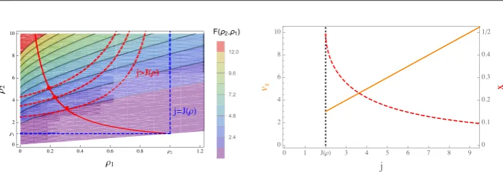
(31) This result has been applied heuristically in [4] for ASEP, and recently in [21] for totally asymmetric ZRPs with concave J(ρ), to derive the large deviation rate function for current fluctuations (22). For fixed, large system size L, lower current deviations on a ring are realized by phase separated travelling wave step profiles with two densities ρ1< ρ2, as illustrated in
figure 1 (top). The probabilistic cost to realize such a profile does not depend on system size since only the non-entropic shock has to be stabilized, which is a localized object. This cost is equal to the entropy production across the reversed stable shock given by F(ρ1,ρ2), which is
equal to −F(ρ2,ρ1) by obvious symmetry in (30).
Travelling wave profiles consist of two phase separated regions with densities ρ1< ρ2.
Denoting by x∈[0, 1] the volume fraction of the high density phase, such a profile has typical current j given by
j= (1−x)J(ρ1) +xJ(ρ2) ρ= (1−x)ρ1+xρ2,
as illustrated in figure 1 (bottom), where ρ denotes the average density associated to the pro-file. By eliminating the variable
x= j−J(ρ1) J(ρ2)−J(ρ1),
(33)
the constraints (32) can be re-written as
G(ρ1,ρ2):= ρ(J(ρ2)−J(ρ1))ρ −J(ρ2)ρ1+J(ρ1)ρ2
2−ρ1 =j.
(34)
This implicitly defines a one-parameter family of admissible densities (ρ1,ρ2) for travelling
wave profiles with given ρ and j=J(ρ), which can often be solved explicitly in paricular cases such as the IPs (see section 3). We consider models where the current-density relation J(ρ) is convex or concave over the whole density region, and it is clear from figure 1 that admissible densities only exist if j>J(ρ) or j<J(ρ), respectively.
Due to this convexity (concavity) assumption, one of the shocks in a travelling wave profile is stable, and the large deviation cost of the profile is given by the negative entropy production across the non-entropic shock. Due to symmetry of the functional (30) we can write this in gen-eral as |F(ρ1,ρ2)|. The associated rate function for fixed total density ρ is then given by
mini-mizing (30) subject to the constraint (34) over all possible density pairs ρ1ρρ2, that is
Etw(j):= inf
ρ1ρρ2
|F(ρ1,ρ2)| : G(ρ1,ρ2) =j∈[0,∞].
(35)
Depending on the specifics of F and G in a given example, the minimizer in (35) is often unique and in the interior of the density domain, and can be found using standard Lagrange multipliers as we will see later. But the global minimum can also be attained at the boundary, as is the case for certain condensing systems as discussed in section 4.2 and in more detail in [21]. If for a given j the condition (34) cannot be fulfilled the minimization in (35) leads to
Etw(j) =∞, and such a current deviation cannot be realized with a travelling wave profile.
There are of course many other strategies to realize large deviations for the empirical cur-rent. Often these involve a global change of the dynamics leading to costs proportional to the system size, and these are only relevant whenever travelling wave profiles are not accessible and discussed for particular cases in later sections. One particular strategy also of a local nature are condensed profiles, which can have costs independent of the system size in systems with bounded rates, as discussed in more detail in section 4.2 for ZRPs. For systems with either convex or concave J(ρ), travelling wave profiles with more than one up and down shock are more costly than the simple one shown in figure 1 (top), and do not contribute to typical large deviation events.
3. Totally asymmetric inclusion process
In this section we follow the same arguments presented in [21] to derive the minimal cost of travelling wave profiles and the rate function for IPs (4) under total asymmetry, i.e.
p = 1 − q = 1.
3.1. Upper current deviations via travelling waves
vs(ρ1,ρ2) =d+ρ1+ρ2.
(36) As can be seen from figure 1 (right), all values j>J(ρ) are accessible by travelling wave profiles, whereas j<J(ρ) are not due to convexity of J(ρ). For given ρ and j>J(ρ) we explicitly solve (34) which takes the form
G(ρ1,ρ2) =dρ−ρ1ρ2+ρ(ρ1+ρ2) =j,
(37) to get the monotone increasing relationship
ρ2(ρ1) =j−ρρ(d+ρ1) −ρ1 →
(j
−dρ)/ρ , asρ1 →0 ∞ , asρ1 →ρ .
(38)
To determine the exponential cost in the minimization problem (35), we first find an explicit expression for the entropy production (30). We find the thermodynamic entropy (31) using explicit expressions summarized in (12),
h(ρ) =ρln
ρ
d+ρ
+dln
d
d+ρ
,
(39)
and the corresponding flux from (26)
g(ρ) =ρ
(d+ρ) ln
ρ
d+ρ
−d
.
(40)
So the Jensen–Varadhan rate function (30) for the IP is given by
F(ρ1,ρ2) =d(d+ρ1+ρ2) ln
d
+ρ1 d+ρ2
+ρ1ρ2ln
ρ2(d+ρ1)
ρ1(d+ρ2)
+d(ρ2−ρ1). (41) Since down shocks are stable due to convexity of J(ρ), we have that F(ρ2,ρ1)>0 and the
travelling wave rate function (35) is given by Etw(j) = inf
ρ1ρρ2{F
(ρ2,ρ1):G(ρ1,ρ2) =j} ∈[0,∞)
(42) for all fixed ρ >0 and j>J(ρ). The minimizer (ρo1,ρo2) of the preceding expression can be obtained from the standard system of equations for local minimization under constraints
∂
1F(ρ2,ρ1)∂2G(ρ1,ρ2)−∂2F(ρ2,ρ1)∂1G(ρ1,ρ2) =0
G(ρ1,ρ2) =j ,
(43)
where the first equation can be written explicitly as
(ρ1−ρ2)
ρln
ρ
2
d+ρ2
d+ρ1 ρ1
+dln
d+ρ 1
d+ρ2
=0.
(44)
We notice that of course for ρ1=ρ2 =ρ this minimization condition is satisfied, which
corre-sponds to the stationary regime with j=J(ρ). The solution (ρo1,ρo2) of the optimization prob-lem in (43) for general j>J(ρ) is unique and can be obtained numerically, as is illustrated in figure 2 together with the plots of the optimal shock speed vs(ρo1,ρo2) and volume fraction of the high density phase (33).
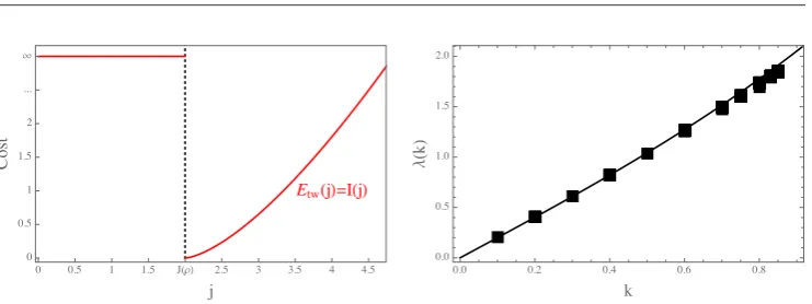
Substituting the solution (ρo1,ρo2) in the JV function F(ρo2,ρo1) for values j>J(ρ) gives rise to a monotone increasing cost function Etw(j), illustrated in figure 3, together with its
L. Therefore, our first main result is that the large deviation rate function (22) in the limit L→ ∞ is given by
I(j) =
E
tw(j), forjJ(ρ) ∞, forj<J(ρ),
(45)
with Etw(j) from (42).
3.2. Predictions for lower current deviations
As discussed in detail in [21] for ZRPs, a generic candidate for a phase separated profile to realize lower current deviations, irrespective of convexity of the flux function, is a condensed profile. This still holds for the IP, if a macroscopic number of particles concentrates on a fixed single lattice site we observe a lower bulk density of the system, and therefore the empirical current is also lower. To achieve a current j<J(ρ) we require a bulk density
R(j) = 1 2
d2+4j−d< ρ,
(46)
simply given by the inverse of J(ρ) in (17), which is strictly increasing in j. Therefore the occupation number of the condensate is of order L(ρ−R(j)) and in order to stabilize it, the exit process from the condensate site has to be unusually slow. Its typical rate is of order L(ρ−R(j))(d+ρ), and the empirically observed rate should be equal to the conditional cur-rent j. As explained in detail in [21], the associated cost EL
c(j) to leading order in L is given by the standard formula to slow down a Poisson process from the typical exit rate to the target rate j, which is given by
EL
c(j) =L(ρ−R(j)) (d+R(j))−j+jlnL(ρ j
−R(j)) (d+R(j)). (47)
Therefore, we have for diverging system size
ec(j):= lim L→∞
EL c(j)
L = (ρ−R(j)) (d+R(j))
[image:12.595.100.468.81.209.2]=ρ(d+R(j))−j (48)
which is positive for all j<J(ρ) and vanishes as jJ(ρ). Note that the condensate can be interpreted as a boundary site with exit rate j, fixing the typical current in the bulk. Then the exit rate at the right end of the bulk into the condensate site is also increased. But since with J(ρ)>0 all characteristic velocities are strictly positive, this only leads to a finite range boundary layer in the bulk density profile. This does not influence the overall current on a macroscopic scale, and therefore does not enter the cost in the rate function.
Another simple strategy to achieve a lower current deviation is to slow down the current across all bonds, independently, from J(ρ) to j<J(ρ). Again this leads to a cost EL
i propor-tional to L, which to leading order is given by
ei(j):= lim L→∞
EL i(j)
L =J(ρ)−j+jln j J(ρ).
(49)
For IPs the jump rates across a bond depend on both adjacent occupation numbers, sug-gesting hyperuniform states with alternating density profiles as further candidates to realize current large deviations (in analogy to results for exclusion [9]). The simplest candidate is a profile alternating between densities ρ1ρρ2 with ρ1+ρ2=2ρ. This corresponds to two
typical currents across even and odd bonds, ρ1(d+ρ2)< ρ2(d+ρ1). To stabilize this, we
need to slow down the higher of both currents to the lower one across all odd or even bonds. Eliminating one variable via ρ1=2ρ−ρ2, the target current for this profile can be written as
j=ρ1(d+ρ2) =2dρ+ (2ρ−d)ρ2−ρ22.
(50) The resulting cost per site, in the limit L→ ∞, is given by
ea(j) =1 2
ρ2(d+ρ1)−j+jln j
ρ2(d+ρ1)
=1 2
ρ2(j) (d+2ρ−ρ2(j))−j+jln j
ρ2(j) (d+2ρ−ρ2(j))
, (51)
[image:13.595.100.471.79.218.2]where the prefactor 1/2 takes into account that only half of the bonds are slowed down and (50) uniquely determines ρ2(j)ρ as
Figure 3. For an IP with ρ=1 and d = 1 we plot the rate function I(j) given in (45) on the left, and the corresponding SCGF on the right. Black diamond data points are obtained from a cloning algorithm simulation [46] with system size L = 128, running time L and 215 clones. Error bars are of the size of the symbols. Discrepancies for large values of k relate to underestimation of rare event probabilities due to finite time sampling, which is a generic feature of large deviation numerics.6
ρ2(j):=12
2ρ−d+(d+2ρ)2−4j.
(52)
We can check that these profiles in fact gives rise to currents j<J(ρ) by differentiating the right-hand side of (50),
dj
dρ2 =2ρ−d−2ρ2 <0 for allρ2ρ.
(53)
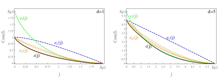
Optimizing over the strategies mentioned above, our (heuristic) prediction for the rate function per volume for lower current deviations j<J(ρ) is given by the lower convex hull
ι(j):=conv{ea(j),ec(j),ei(j)} asL→ ∞,
(54) as illustrated in figure 4.
Our ansatz for the alternating profiles assumes product measures with alternating densities. In general, other hyperuniform states with long range correlations might have a different cost, but still proportional to the system size. So strictly speaking, (54) is only an upper bound for the rate function, but we have good reason to believe that we considered all relevant strategies to realize current large deviations. Firstly, since the condensed cost (47) scales linearly with the size of the condensate to leading order, any split of the excess mass into several macro-scopic isolated clusters will lead to the same total cost to leading order and therefore to (48). Secondly, it turns out that all other profiles with periodic spatial patterns have higher cost than
ea( j ), as follows: if we assume that the lowest density in a single period of the profile is R(j)
as given in (46), all bonds that have a stationary rate larger than j must be slowed down to a rate
j. The cost of slowing down these Poisson processes to rate j as a function of the excess mass above R(j), is given by the usual rate function analogous to (51) and is subadditive. It follows that periodic configurations of period m are all at least as costly as having a single highly occupied site followed by m − 1 sites with density R(j). Furthermore, this cost is increasing in m, as illustrated in figure 4. This follows from another straightforward calculation, using the convexity of the cost of slowing the appropriate stationary jump rate, with j fixed as a function of the high density ρ2(j), and the fact that for m3 this density and the analogue of (50) take a particularly simple form; j=ρ1(d+ρ1) and ρ2(j) =mρ−(m−1)R(j).
We see in figure 4, for two different parameter values d, that in general the alternating cost
ea( j ) is always below the condensed cost ec( j ), coinciding only for j = 0 an J(ρ). For j only
slightly below J(ρ) the dominating strategy is to slow down all bonds, whereas for smaller val-ues of j the alternating profile becomes dominant, leading to a rate function given by the lower convex hull of both curves. So our heuristic considerations predict a dynamic phase transition for lower current large deviations in IPs for large system sizes. Since the rate functions are of order L and the rates of the IP are unbounded, these predictions are currently beyond verifica-tion with numerical methods which have been used to produce the data in figure 3.
4. Partially asymmetric systems
systems, we will illustrate it for condensing ZRPs, which allow for the most interesting behav-iour in this class of models, due to the interplay between travelling wave and condensed profiles.
4.1. Travelling wave and condensed profiles
To set the notation, we recall the general expression of stationary currents for systems with product measures in section 2 and note that for partial and total asymmetry they are simply related as
JPA(ρ) = (p
−q)JTA(ρ),
(55) where we use the labels PA and TA in the superscript to distinguish systems with
p(x,y) =pδy,x+1+qδy,x−1 and p(x,y) =δy,x+1, respectively. We notice that the stationary
measure (5), the relation R(φ) (9) and its inverse Φ(ρ) are unaffected by the partial asym-metry. Recalling (31), this implies that the thermodynamic entropy h(ρ) remains unchanged. Using (26) we can determine the corresponding entropy flux g(ρ) and get
hPA(ρ) =hTA(ρ) and gPA(ρ) = (p
−q)gTA(ρ) .
(56) From (30), the Jensen–Varadhan functional for partially asymmetric systems is then simply given by
FPA(ρ1,ρ2) = (p−q)FTA(ρ1,ρ2).
(57) Again, in the same way, the consistency condition for travelling wave profiles (34) becomes
GPA(ρ
1,ρ2) = ρ
JPA(ρ
2)−JPA(ρ1)−JPA(ρ2)ρ1+JPA(ρ1)ρ2 ρ2−ρ1
(58)
= (p−q)GTA(ρ1,ρ2) =j.
[image:15.595.97.470.85.219.2]The optimization expression for the cost function (35) can then be used to determine its par-tially asymmetric counterpart,
EPA
tw (j) =ρ inf 1ρρ2
FPA(ρ1,ρ2):GPA(ρ1,ρ2) =j
=(p−q) inf ρ1ρρ2
FTA(ρ1,ρ2):GTA(ρ1,ρ2) =j/(p−q)
=(p−q)ETA
tw
j
p−q
. (60)
In analogy to (47), recalling that for partial asymmetry the bias across each bond is multi-plied by (p−q), we can write the cost of a condensed profile as
EPA
c (j) = (p−q)u((ρ−R(j))L)−j+jln(p j
−q)u((ρ−R(j))L) . (61) Pulling out the factor (p−q) it is easy to see that the same scaling relationship as for EPA
tw
holds in general for condensed states, i.e.
EPA
c (j) = (p−q)ETAc
j
p−q
.
(62)
We will use this general understanding of the effects of partial asymmetry on costs of travel-ling wave and condensed profiles in the next subsection and apply it to condensing ZRPs.
Note that in the above derivation we do not make use of the factorized form of stationary states. The only important ingredient is that states, and their associated entropy, are independ-ent of the bias (p,q). Then the above relation between costs for partially and totally asym-metric systems holds.
4.2. Partially asymmetric ZRPs
We will illustrate the general result of the previous section for lower current deviations for a condensing ZRP with rates
u(0) =0, u(n) =1+b/n for alln1 .
(63) This model has been widely studied in the literature (see e.g. [31, 43, 53]). It is known to have a concave flux function, and in [21] we derived the current large deviation function for the totally asymmetric version of the process. It exhibits a dynamic phase transition, where for certain parameter values the rate function is determined by condensed states rather than travelling waves for small enough j, as is shown in figure 5. For the rates (63) we have u((ρ−R(j))L)1, as L→ ∞, to leading order, and therefore the condensed cost (62) sim-plifies to
EPA
c (j)(p−q)
1−p j −q +
j p−qln
j p−q
.
(64)
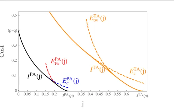
This asymptotic behaviour is independent of L since the rates of the process are bounded, in contrast to the IP. The main result in [21] states that the rate function for lower current devia-tions in any ZRP with concave flux function is the lower convex hull of ETA
tw and EcTA. With (60) and (62) the same is true for partially asymmetric systems, i.e.
IPA(j) =convEPA
tw,EcPA(j) for all 0<j<J(ρ), ifρc<∞
for condensing systems, and IPA(j) =EPA
tw(j) for all 0<j<J(ρ), ifρc=∞
(66) for non-condensing systems. In particular, we can relate the full rate function, IPA, to the
totally asymmetric one for general ZRPs, using the scaling derived above, as
IPA(j) = (p
−q)ITA j p−q
,
(67)
which is illustrated in figure 5 for the particular example with rates (63). The travelling wave cost for p = 1 − q = 1 has been evaluated numerically for the given parameter values in [21], in analogy to the procedure outlined in section 3 for the IP. We do not discuss details of the shape of the cost and rate function here, which can be found in [21]. In figure 6 we numer-ically confirm this result by comparing simulation data to the SCGF λ(k), predicted as the
Legendre transform of the rate function IPA( j ).
4.3. Beyond phase separated states
In general, outside the accessible range of conditional currents for travelling wave or con-densed profiles (which is 0<j<J(ρ) for ZRPs with concave flux function), we expect the cost for current large deviations to scale with the system size as explained in section 3.2 for the IP. The presence of partial asymmetry introduces additional randomness and allows fluctua-tions also at the level of the spatial part of the dynamics. In fact, it is possible to reach a target current j, conditioning on an empirical bias (p,q) with
(p−q) Φ (ρ) =j and p+q=1,
(68) which implies
p(j) =j+ Φ (ρ) 2Φ (ρ) .
[image:17.595.158.437.81.256.2]Due to the obvious constraints p,q∈[0, 1] on the spatial coefficients, it is possible to achieve a bounded set of currents j∈−JTA(ρ),JTA(ρ) by conditioning purely on an empirical bias, and leaving the jump rates in the process unchanged. In particular, due to the additional ran-domness from partial asymmetry, the system may obtain atypical fluctuations of the current in the direction opposite to the stationary current. The cost to alter the empirical bias across the whole system is of order L (since it independently accrues at each bond) and diverges with the system size. The cost to condition on an atypical spatial bias per bond is given by the relative entropy, which is the standard rate function for observing an empirical bias (p,q), given the true bias (p,q) (see e.g. [54]), which leads to
epq(j):= Φ (ρ)
p(j) lnp(j)
p +q(j) ln q(j)
q
.
(70)
To complete the picture, it is possible to achieve currents beyond the interval
−JTA(ρ),JTA(ρ) by increasing also the empirical jump rates of the model. In fact, using the same reasoning as for the condensed case in (64), increasing the empirical exit rate of the particles Φ (ρ), has a cost function per site given by the acceleration of a Poisson process from Φ (ρ) to a value φ >ˆ Φ (ρ)
eΦ
ˆ
φ:= Φ (ρ)−φˆ+ ˆφln φˆ Φ (ρ).
(71)
Keeping the asymmetry (p,q) fixed, this mechanism in isolation with j= (p−q) ˆφ would lead to a cost function per volume
eJ(j):= (p−q)eΦ
ˆ
φ=j−JPA(ρ) +JPA(ρ) lnJ PA(ρ)
j ,
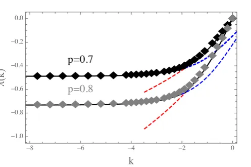
[image:18.595.160.409.88.253.2](72) Figure 6. SCGF (black line) given by (23) as L→ ∞ for a partially asymmetric ZRP with rates (63) where b = 3.5, ρ=0.25 and p = 0.7 and 0.8, resulting from Legendre transform of the rate function (65). Data points obtained from a simulation using the cloning algorithm (with 215 clones, L = 64 and running time L2). The red (blue) dashed curve is the Legendre transform of the travelling wave (condensed) cost functions EPA
tw(j) (and EPAc (j)). The resulting kink corresponds to the dynamic transition between travelling wave and condensed profiles. Error bars are of the size of the symbols.7
where JPA(ρ) = (p
−q) Φ (ρ). In general the two mechanisms (70) and (72) can interact. For instance, to obtain an atypical negative current, the system needs to change the spatial bias, but it may be more efficient to combine this with an additional increase of the empirical exit rate. Along the same lines, reaching a current above JPA(ρ) can be achieved as a combination of increasing the asymmetry of the spatial part and the system activity. Adding both costs with
(p−q) ˆφ=j and thus pj,φˆ= j+ ˆφ 2φˆ ,
(73)
leaves only φˆ as a free parameter to optimize. This leads to the combined optimal cost
epq;J(j):= min
ˆ
φΦ(ρ)
ˆ
φ
pj,φˆlnp j,φˆ
p +q
j,φˆlnq j,φˆ
q
+ (p−q)
Φ (ρ)−φˆ+ ˆφln φˆ
Φ (ρ) . (74)
Finally, we denote the cost per volume of the L-independent rate function (67) due to phase-separated profiles as
ιPA(j) = lim L→∞
IPA(j)
L =
0, j
∈0,JPA(ρ)
∞, otherwise .
(75)
Then our prediction for the rate function per volume for any j∈R can be written as the con-vex hull
ι(j):=convepq;J,ιPA(j) for allj∈R.
(76) The plot of all relevant cost functions and the resulting rate function can be found in figure 7. For small and large values of j the rate function is dominated by the combined cost epq;J( j ),
but vanishes for the whole interval j∈[0,JPA(ρ)], due to the size-independent cost of phase separated profiles described in the previous subsection. This leads to a dynamic transition for negative j close to the origin, corresponding to a mixture of fully condensed profiles with van-ishing current and homogeneous ones with global change of activity/bias and negative current. We obtain the corresponding SCGF by Legendre–Fenchel transform of (76), which is shown in figure 8 in comparison with simulation data. This is possible here, in contrast to results in section 3.2 for IPs, since the rates of the ZRP we consider are bounded. The two affine parts of the rate function turn into kinks, while the kink at j = 0 turns into the flat part of the SCGF. Since the large deviation speed now scales with L, the SCGF (23) has to be rescaled as
1
LλL(kL)→λ∞(k) asL→ ∞,
(77)
to compare data with tilt parameter kL to the asymptotic behaviour.
rate function (76) only depend on macroscopic features, and can in principle be computed for much more general models. However, as we have seen in section 3.2 for the IP, microscopic features of the system can lead to other profiles contributing to the rate function, and (76) is not a completely general expression. Still, for models with finite correlation lengths in the Figure 7. Large deviation rate function ι(j) (76) per volume (black) for a partially asymmetric ZRP with rates (63) where b = 3.5, ρ=0.25 and p = 0.7. The cost of travelling wave profiles for j∈[0,JPA(ρ)] vanishes on the scale L, leading to a dynamic transition from phase separated profiles to global activity and bias conditioning, as explained in the text. These qualitative features of the plot are independent of the choice of jump rates (which would only shift the position of JPA). The cost epq;J( j ) optimizing between spatial and activity contribution given in (74) (full red line) does not coincide with epq( j ) (70) (dashed orange) nor eJ( j ) (72) (dashed blue).
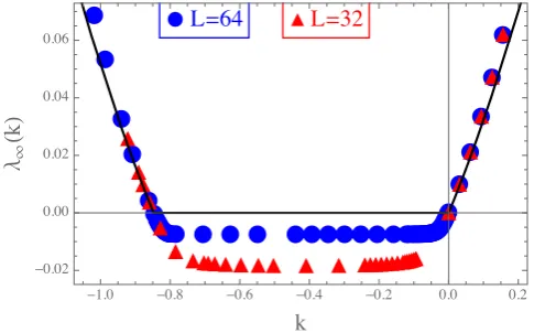
Figure 8. SCGF λ∞(k) normalized by the system size (black line) given by (77), corresponding to the rate function (76) for the same ZRP as in figure 7. Data points are obtained from a simulation using the cloning algorithm with 215 clones, L2 running time and system size L = 32 (red), L = 64 (blue). The discrepancy between the data points and λ∞(k) is due to a generic finite size effect smoothing kinks and affine parts of the function, which decreases with L. Note that the fluctuation relation (78) holds as explained in the text with V= lnp/q≈0.847. Error bars are of the size of the symbols.8
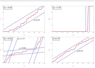
[image:20.595.155.398.367.518.2]stationary state and concave flux-density relation, we expect the rate function to show the same qualitative behaviour and in particular to exhibit a crossover between local phase sepa-rated profiles and global conditioning. Typical profiles contributing to data points in figure 8
for different values of k are shown in figure 9.
In figure 8 it is clearly visible that the generalized fluctuation relation for the current [55–57] is obeyed by the system, which translates into a corresponding symmetry property of the SCGF
λL(k) =λL−k−VL for allk∈Rand withV := lnp q .
(78)
As explained in [57], the parameter V/2 can be interpreted as the field per volume driving the original system, which has to be reversed to achieve a negative current deviation. Note that V and therefore the symmetry (78) is entirely independent of the rates u(n) of the process.
5. Discussion
[image:21.595.101.471.78.342.2]We explore the general applicability of a recent approach [21] to study current large deviations in periodic particle systems with unbounded local occupation number. We cover extensions to convex current-density relations and also partially asymmetric dynamics, which we illus-trate for IPs and ZRPs. In addition to phase separated profiles, which lead to rate functions
Figure 9. Typical integrated profiles σx:=yxηy (red full lines) that contribute to data points in figure 8 for different values of k, using the same ZRP as in figure 7. Dashed blue lines illustrate the corresponding densities ρ=0.25 for flat profiles with k = −0.94 and 0.19, the optimal pair (ρ1,ρ2) for travelling wave profiles for k = −0.02 minimizing (35), and the condensate for k = −0.7.9
independent of the system size in a restricted range of currents, we also predict extensive rate functions outside this range. While the particular profiles contributing to the extensive costs depend on the particular model (as illustrated here for IPs and ZRPs), the qualitative features of the resulting extensive rate function (see figure 7) are expected to be quite generic: vanishing for currents accessible by phase separated profiles, and an associated crossover to extensive costs. As mentioned in the introduction, this feature has been pointed out before for several models [22–29].
We have also established a general relationship between partially and totally asymmetric costs for travelling wave and condensed profiles. This holds for any model where the station-ary state (whether it factorizes or not) does not depend on the bias of the dynamics. Whenever the stationary state has finite correlation lengths travelling wave profiles provide size-inde-pendent costs to realize large deviations in a restricted range of currents, depending on the convexity properties of the current-density relation. The approach based on Jensen–Varadhan theory is expected to apply also for non-factorized steady states, and in this case the thermo-dynamic entropy would be characterized by the thermothermo-dynamic limit of canonical entropies
1
LlogZL,N→h(ρ) asL,N→ ∞, N/L→ρ.
Existence of this limit would be a minimal prerequisite to apply the approach at least on a heu-ristic level. In this context Katz–Lebowitz–Spohn models [58] which have explicitly known non-factorized states of nearest-neighbour Gibbs type provide a promising class to further test the applicability of this approach. The current-density relations of those systems are also known to exhibit convex and concave regions for certain parameter values, leading to interest-ing phase diagrams for open boundaries [59]. While fully concave or convex current-density relations are covered in the present paper, the interplay between convex and concave regions is likely to lead to interesting effects for travelling wave profiles.
Acknowledgments
AP acknowledges support by the Engineering and Physical Sciences Research Council (EPSRC) Grant No. EP/L505110/1, by The Alan Turing Institute EPSRC grant EP/N510129/1 and seed project SF029 ‘Predictive graph analytics and propagation of information in net-works’, by National Group of Mathematical Physics (GNFM-INdAM), by Imperial College together with the Data Science Institute and Thomson-Reuters Grant No. 4500902397-3408.
ORCID iDs
Paul Chleboun https://orcid.org/0000-0003-0387-3432
Stefan Grosskinsky https://orcid.org/0000-0002-5113-9112
Andrea Pizzoferrato https://orcid.org/0000-0002-7334-0685
References
[1] Lazarescu A 2015 The physicist’s companion to current fluctuations: one-dimensional bulk-driven lattice gases J. Phys. A: Math. Theor. 48 503001
[3] Gorissen M, Lazarescu A, Mallick K and Vanderzande C 2012 Exact current statistics of the asymmetric simple exclusion process with open boundaries Phys. Rev. Lett. 109 170601 [4] Bodineau T and Derrida B 2006 Current large deviations for asymmetric exclusion processes with
open boundaries J. Stat. Phys. 123 277–300
[5] Derrida B 2007 Non-equilibrium steady states: fluctuations and large deviations of the density and of the current J. Stat. Mech. P07023
[6] Harris R J, Rákos A and Schütz G M 2005 Current fluctuations in the zero-range process with open boundaries J. Stat. Mech. P08003
[7] Harris R J, Popkov V and Schütz G M 2013 Dynamics of instantaneous condensation in the ZRP conditioned on an atypical current Entropy 15 5065–83
[8] Hirschberg O, Mukamel D and Schütz G M 2015 Density profiles, dynamics, and condensation in the ZRP conditioned on an atypical current J. Stat. Mech. P11023
[9] Popkov V, Schütz G M and Simon D 2010 ASEP on a ring conditioned on enhanced flux J. Stat. Mech. P10007
[10] Tsobgni N P and Touchette H 2016 Large deviations of the current for driven periodic diffusions Phys. Rev. E 94 032101
[11] Gupta S, Barma M and Majumdar S N 2007 Finite-size effects on the dynamics of the zero-range process Phys. Rev. E 76 060101
[12] Tizón-Escamilla N, Lecomte V and Bertin E 2018 Effective driven dynamics for one-dimensional conditioned Langevin processes in the weak-noise limit (arXiv:1807.06438)
[13] Bertini L, De Sole A, Gabrielli D, Jona-Lasinio G and Landim C 2015 Macroscopic fluctuation theory Rev. Mod. Phys. 87 593
[14] Bertini L, Faggionato A and Gabrielli D 2015 Large deviations of the empirical flow for continuous time markov chains Ann. Inst. Henri Poincare B 51 867–900
[15] Bertini L, Faggionato A and Gabrielli D 2015 Flows, currents, and cycles for markov chains: large deviation asymptotics Stoch. Process. Appl. 125 2786–819
[16] Smoller J 1994 Shock Waves and Reaction–Diffusion Equations (Berlin: Springer)
[17] Varadhan S R S 2004 Large deviations for the asymmetric simple exclusion process Stochastic Analysis on Large Scale Interacting Systems (Adv. Studies Pure Math. vol 39) ed T Funaki and H Osada (Tokyo: Math. Soc. Japan) pp 1–27
[18] Jensen L H 2000 Large deviations of the asymmetric simple exclusion process in one dimension PhD Thesis New York University
[19] Vilensky Y 2008 Large deviation lower bounds for the totally asymmetric simple exclusion process PhD Thesis New York University
[20] Derrida T Bodineau B 2005 Distribution of current in nonequilibrium diffusive systems and phase transitions Phys. Rev. E 72 066110
[21] Chleboun P, Grosskinsky S and Pizzoferrato A 2017 Lower current large deviations for zero-range processes on a ring J. Stat. Phys. 167 64–89
[22] Derrida B and Lebowitz J L 1998 Exact large deviation function in the asymmetric exclusion process Phys. Rev. Lett. 80 209–13
[23] Derrida B and Appert C 1999 Universal large-deviation function of the Kardar–Parisi–Zhang equation in one dimension J. Stat. Phys. 94 1–30
[24] Bodineau T, Derrida B, Lecomte V and van Wijland F 2008 Long range correlations and phase transitions in non-equilibrium diffusive systems J. Stat. Phys. 133 1013–31
[25] Prolhac S and Mallick K 2009 Cumulants of the current in a weakly asymmetric exclusion process J. Phys. A: Math. Theor. 42 175001
[26] Espigares C P, Garrido P L and Hurtado P I 2013 Dynamical phase transition for current statistics in a simple driven diffusive system Phys. Rev. E 87 032115
[27] Baek Y, Kafri Y and Lecomte V 2018 Dynamical phase transitions in the current distribution of driven diffusive channels J. Phys. A: Math. Theor 51 10
[28] Tizón-Escamilla N, Pérez-Espigares C, Garrido P L and Hurtado P I 2017 Order and symmetry breaking in the fluctuations of driven systems Phys. Rev. Lett. 119 090602
[29] Lazarescu A 2017 Generic dynamical phase transition in one-dimensional bulk-driven lattice gases with exclusion J. Phys. A: Math. Theor. 50 254004
[30] Drouffe J-M, Godrèche C and Camia F 1998 A simple stochastic model for the dynamics of condensation J. Phys. A: Math. Gen. 31 L19
[32] Evans M R and Hanney T 2005 Nonequilibrium statistical mechanics of the zero-range process and related models J. Phys. A: Math. Gen. 38 R195
[33] Godrèche C 2007 From Urn models to zero-range processes: statics and dynamics Lecture Notes Phys. 716 261–94
[34] Godrèche C and Luck J-M 2012 Condensation in the inhomogeneous zero-range process: an interplay between interaction and diffusion disorder J. Stat. Mech. P12013
[35] Chleboun P and Grosskinsky S 2014 Condensation in stochastic particle systems with stationary product measures J. Stat. Phys. 154 432–65
[36] Giardinà C, Kurchan J, Redig F and Vafayi K 2009 Duality and hidden symmetries in interacting particle systems J. Stat. Phys. 135 25–55
[37] Grosskinsky S, Redig F and Vafayi K 2013 Dynamics of condensation in the symmetric inclusion process Electron. J. Probab. 18 1–23
[38] Chau Y, Connaughton C and Grosskinsky S 2015 Explosive condensation in symmetric mass transport models J. Stat. Mech. P11031
[39] Jack R L, Thompson I R and Sollich P 2015 Hyperuniformity and phase separation in biased ensembles of trajectories for diffusive systems Phys. Rev. Lett. 114 060601
[40] Karevski D and Schütz G M 2017 Conformal invariance in driven diffusive systems at high currents Phys. Rev. Lett. 118 030601
[41] Andjel E D 1982 Invariant measures for the zero range process Ann. Probab. 10 525–47
[42] Balázs M, Rassoul-Agha F, Seppäläinen T and Sethuraman S 2007 Existence of the zero range process and a deposition model with superlinear growth rates Ann. Probab. 35 1201–49 [43] Grosskinsky S, Redig F and Vafayi K 2011 Condensation in the inclusion process and related
models J. Stat. Phys. 142 952–74
[44] Touchette H 2018 Asymptotic equivalence of probability measures and stochastic processes J. Stat. Phys. 170 962–78
[45] Bodineau T and Derrida B 2004 Current fluctuations in nonequilibrium diffusive systems: an additivity principle Phys. Rev. Lett. 92 180601
[46] Giardinà C, Kurchan J, Lecomte V and Tailleur J 2011 Simulating rare events in dynamical processes J. Stat. Phys. 145 787–811
[47] Kipnis C and Landim C 2013 Scaling Limits of Interacting Particle Systems vol 320 (Berlin: Springer)
[48] Bahadoran C, Guiol H, Ravishankar K and Saada E 2017 Constructive euler hydrodynamics for one-dimensional attractive particle systems (arXiv:1701.07994)
[49] Stamatakis M G 2015 Hydrodynamic limit of mean zero condensing zero range processes with sub-critical initial profiles J. Stat. Phys. 158 87–104
[50] Opoku A and Redig F 2015 Coupling and hydrodynamic limit for the inclusion process J. Stat. Phys. 160 532–47
[51] Schütz G M and Harris R J 2007 Hydrodynamics of the zero-range process in the condensation regime J. Stat. Phys. 127 419–30
[52] Lax P D 1973 Hyperbolic Systems of Conservation Laws and the Mathematical Theory of Shock Waves (Philadelphia: SIAM)
[53] Giardinà C, Redig F and Vafayi K 2010 Correlation inequalities for interacting particle systems with duality J. Stat. Phys. 141 242–63
[54] Den Hollander F 2008 Large Deviations vol 14 (Providence, RI: American Mathematical Society) [55] Lebowitz J L and Spohn H 1999 A Gallavotti–Cohen type symmetry in the large deviation
functional for stochastic dynamics J. Stat. Phys. 95 333–65
[56] Harris R J, Rákos A and Schütz G M 2006 Breakdown of Gallavotti–Cohen symmetry for stochastic dynamics Europhys. Lett. 75 227
[57] Rákos A and Harris R J 2008 On the range of validity of the fluctuation theorem for stochastic markovian dynamics J. Stat. Mech. P05005
[58] Katz S, Lebowitz J L and Spohn H 1984 Nonequilibrium steady states of stochastic lattice gas models of fast ionic conductors J. Stat. Phys. 34 497–537