Abstract— The congestion control problem in data networks
is analyzed here from the point of view of control systems, and some solutions are compared. By analyzing in detail their linearized transfer functions, it is discussed why TCP Westwood and TCP NewReno present different behavior when dealing with the same network conditions, showing why TCPWestwood gives better performance. Moreover it is shown that adequate stability and performance can be obtained, even in the presence of the wide variations in the parameters of the networks, as long as the controller is properly designed.
Index Terms— congestion control, control systems, robust
performance, TCP Westwood, TCP NewReno, transfer function.
I. INTRODUCTION
outers are central components in modern data networks, as they simplify the connection of several networks, directing data to the final destination. When the router receives more data than the maximum limit it can process then congestion happens, causing excessive transmission delays, blocking of new connections, and losses of packets (see, for example, [1], [3], and references therein). If this congestion is not properly treated congestive collapse occurs, with the router providing very low throughput.
To correct this problem modern routers implement protocols that include some congestion control techniques, which provide feedback to the previous nodes in the network, in order for them to adapt the traffic to the maximum capacity of the congested router (see, for example, [4], [5]). This feedback is frequently provided by dropping packets: when the loss of some packets in a data link is detected, the protocols implemented in previous nodes reduce the traffic. Many congestion control algorithms have been proposed: this paper concentrates on those implemented in two of the most popular protocols: We assume that the protocol implemented at the transport layer is the Transmission Control Protocol (TCP), with an Active Queue Management (AQM) algorithm implemented in the network scheduler within the routers. These AQM algorithms implement the congestion control algorithm: a queue is implemented at the interface with each link, that holds the packets that have being scheduled (by TCP) to go
Manuscript received March 2014. Work funded by MiCInn DPI2010-21589-C05-05.
T. Alvarez, H. de las Heras and J. Reguera are with the University of Valladolid (Telf: +34 983423162; email: [email protected]).
out in that link; before the queue is full, in order for the sender to detect the congestion problem as soon as possible some packets are dropped (or marked, depending on the specific algorithm) [5,6]. Compared with other congestion control algorithms (such as the drop-tail implemented in many routers), AQM marks the packets probabilistically to improve sharing the bandwidth between different links, the improving the processing of bursty flows and avoiding synchronized oscillations between the links.
Many AQM algorithms have been proposed and tested (see, for example, [5]). Moreover, even if the same AQM technique is implemented results are different depending on the TCP protocol used. This paper concentrates on discussing the advantages of using algorithms derived from techniques that are standard in control systems and have being extensively tested in application areas other than data networks (see [7,8] for some general reference of control systems in general) considering two different TCP variants: Westwood and New Reno. These control system techniques normally require an approximate model of the system to be controlled, expressed as linear dynamic transfer function; some dynamical models of data congestion were already proposed in [10], and its linearization was discussed in [10].
From the many controller design methodologies proposed in control systems, PID control is probably the most widely used to develop AQM algorithms. We can cite [12], [13], [14], [15] and references therein.
In order to make these studies the methodologies described will be applied to a specific communication problem: using simulation would make possible to make a fair comparison, by reproducing the same traffic conditions when testing each algorithm.
This paper will present a comparison between Westwood TCP and NewReno TCP. The non linear fluid models are linearized and the transfer function models are then obtained. These transfer functions will be compared using the step response, the frequency response, the location of poles and zeros under different network configurations. These studies will help to understand why TCP Westwood behaves better when there are changes in the traffic conditions, number of users or delay in the network, regardless of the type of communication (wired or wireless).
The organization of the paper is the following: Sections 2 and 3 describe the TCP Westwood and TCP NewReno protocol and their fluid models. Section 4 presents a comparison between TCP Westwood and TCP NewReno.
Controller Design for Congestion Control:
Some Comparative Studies
Teresa Alvarez, Hector de las Heras, Javier Reguera
and finally Section 6 discusses some experiments. A discussion concludes the paper.
II. TCPWESTWOOD
TCP Westwood (TCPW) [16] is a popular congestion control algorithm that has shown to provide robust selections for the congestion control parameters (in fact, it is implemented with minor modifications as part of the Linux kernel). It is particularly relevant when packet losses are not only generated by congestion control algorithms (for example in wireless networks).
TCPW relies on studying the stream of returning acknowledgment packets (ACKs) to adapt some parameters of the congestion control algorithm [16], in particular the size of the so-called congestion window (cwnd) that fixes the maximum number of bytes that can be accepted at each link: this window is slowly increased until some acknowledgements are not received or a timeout expires.
A. Fluid-flow Model
The nonlinear dynamical model of TCPW ([15], [16], [17], [18]) is now presented, as it will be the base of the models used for controller design and comparison. If W(t) denotes the size of the TCPW window at a given link in packets, the number of packets at the corresponding queue (q(t):queue length) can be derived from the following equations as follows:
) ( ) ( ) ( ) ( )
( W t
T t C t q t N t C dt dq p
(1)
()
)) ( ( ) ( ) ( ) ( )) ( ( ) ( ) ( ) ( ) ( ) ( 1 2 t R t p T t R t C t R t q t R t W T t R t p T t R t C t R t q t R t W t W T t C t q dt dW p p p p (2)Where Tp is the propagation delay (in seconds), C(t) is the
link capacity (in packets/s), N(t) is the number of TCPW sessions (load factor) and R(t) is the round-trip time (equal to q(t)/C(t)+Tp) and p(t) is the variable that is modified by the AQM algorithm: the probability of discarding a packet (or marking it in some AQM implementations).
B. Model for controller design
As it has been mentioned, a linear model with constant parameters is frequently used to design control systems, as it simplifies the analysis and design of controllers. This kind of models can be easily derived by linearization: in our case, temporarily assuming that the number of active TCPW sessions, the link capacity and the round-trip time do not change, and discarding high-frequency components, a Taylor approximation of (1) and (2) at a given set of operating parameters gives the following transfer-function description of our system (see [11]or [15] for details):
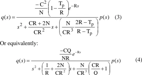
) ( T R T R 2 CR N CR N 2 CR R T 1 N C ) ( p p 3 2 2 R p 2 s p s s e s q s (3) Or equivalently: ) ( 1 Q CR CR N CR N 2 R 1 NR CQ ) ( 3 2 2 R s p s s e s q s (4)
[image:2.595.305.548.53.182.2]Where C, N, R and Q are the values of C(t), N(t), R(t) and q(t) at the current working point.
Figure 1: Block diagram of the AQM feedback control system
The static gain of this linearized system would be:
22 2 2 p 2 p 2 2 3 T 2R T R N R C N Q CR R C Q (5)
With the system responding as a stable second-order system with delay R, underdamped if Tp>2NR.
III. TCP NEWRENO
TCP NewReno (TCPNR) is still probably the most widely used congestion control technique (with several variants), although TCPW provides better performance when the link includes large paths or might generate unexpected packet losses (like wireless networks). This simpler algorithm can be modelled as follows:
) ( ) ( ) ( ) ( )
( W t
T t C t q t N t C dt dq p
(6)
p
t R
T R t C R t q R t W t W T t C t q dt dW p p ) ( ) ( ) ( ) ( 1 (7)The corresponding transfer function model is then
Thus, it can be seen that the TCPNewReno static gain is
and the dynamic response corresponds to a second order overdamped system with delay R, and real poles placed at
R 1 , R C N 2 2
(11) Where the dominant pole is given by -2N/(CR2). Please, take into account that only if 2N/C is bigger than 1/R the dominant pole would be -1/R.
IV. COMPARISON BETWEEN TCPW AND TCPNR Research has shown ([16]) that TCPW is a good approach when there are wireless links in the network. This section presents a comparison using the transfer function models of TCPW and TCPNR in order to achieve some conclusions regarding the static gain, the open loops and the frequency response of each system. This analysis will allow designing adequate controllers. The number of users (N) and the RTT (R) should have coherent values.
In [20] and [21] some guidelines on how to choose these values were given. The best scenario is to have many users and a small delay. The worst situation is to have few users and a big delay. This conclusion is true for both TCP approaches under study.
First, let’s compare the static gain of both systems: - TCPW static gain (5):
22 2 2 N Q CR R C Q
- TCPNR static gain (10): 2 3 3 N 4 R C
Which one is bigger? It depends on the parameters’ values, but (usually) (5) will be bigger than (10), i.e., the input will be amplified:
23 3 2 2 2 2 N 4 R C N Q CR R C Q
Practical examples will show this. This is a very important inference for the designing controllers: when the number of users or the delay change in the network, TCPW will be more robust than TCPNR.
Both systems have no zeros and both have two poles. However, the TCPNR transfer function always has two real poles and the TCPW system’s poles can be real or complex conjugate. The denominators of both transfer functions are:
- TCPW:
1 Q CR CR N CR N 2 R 1 3 2 2 s s - TCPNR: 3 2 2 CR 2N CR N 2 R 1 s s
The second and first order terms are equal, the difference is on the independent, term and they have very similar:
1 Q CR CR N
3 versus CR3
2N
is the same than
1 Q CR versus 2
When is
1 Q CR
greater than 2? It depends on C, R and Q, but in real networks the initial queue length will be smaller than the R times C. As a result, for a given N, C, R and Q, the two poles of TCPW are always placed between the two poles of TCPNR. Another conclusion is that TCPW will be a bit faster than TCPNR. This also can be justified looking at the analytical solution of the poles:
If we look at the solution of the second order equation of TCPNR: 2 CR N 4 R C N 4 R 1 CR N 2 R 1 2 CR 2N 4 CR N 2 R 1 CR N 2 R 1 3 4 2 2 2 2 3 2 2 2 2 , 1 poles
On the other hand, the poles of TCPW will be given by:
2 QR N 4 R C N 4 R 1 CR N 2 R 1 2 1 Q CR CR N 4 CR N 2 R 1 CR N 2 R 1 2 4 2 2 2 2 3 2 2 2 2 , 1 poles
When 2 4
2 2 2 R C N 4 R 1 QR N 4
, then the poles will be complex conjugate.
A second order system is characterized by this equation:
) ( 2
)
( 2 2
2 s p w s w s Kw s q n n n
, where is the damping ratio
and wn the natural frequency.
Considering TCPW: 3 2 2 2 2 2 1 2 1 2 CR N Q CR s CR N R s w s w s NR CQ Kw n n n 3 2 1 CR N Q CR
wn
CR Q
CRN Q N CR
CR N Q
CR CR
N R
2 2
1 2
2 1
3 2
When the poles are complex conjugate:
2 2
,
1 wnjwn 1 poles
V. CONTROLLER DESIGN
This section briefly describes how a controller can be implemented into an AQM approach. Figure 1 shows the basic structure. As it has been mentioned the control action in AQM algorithm is probability of dropping (or marking) packets p(t) , with is adapted by comparing the current queue length q(t) with a desired value qref (a percentage of
the real capacity of the queue): see Figure 1.
We have chosen the PID controller [2] as the AQM congestion control algorithm, as this controller is widely used and gives good results. The structure of the controller is:
t
d i
p
t
d i
p
dt t de K d e K t e K
dt t de T d e T t e K t u
0 0 1
(12)
It must be pointed out that this is the ideal equation: When the controller is implemented, the derivative term should be treated as a first order filter.
VI. EXAMPLES
[image:4.595.319.558.116.264.2]This section compares TCPW and TCPNR under different traffic conditions. The basic topology is depicted in Figure 2. Different scenarios will be considered.
Figure 2: Dumbbell topology
A. First experiment: Fixed N, changing R
The first batch of experiments considers the parameters shown in Table I. We consider a fixed N and a changing R. The greater the delay, the smaller the initial marking probability.
TABLEI NETWORK CONFIGURATIONS
N R C P0 Q
[image:4.595.50.547.490.730.2]Case1 50 0.15 3750 0.0158 200 Case2 50 0.3 3750 0.0040 200 Case3 50 0.6 3750 0.0010 200 Case4 50 0.8 3750 0.0006 200 Case5 50 1.1 3750 0.0003 200
TABLE II. Fixed N, changing R
Caso 1 Caso 2 Caso 3 Caso 4 Caso 5
TCPW tf
06 . 15 852 . 7
100000
2
s
s 3.63 3.272
50000
2
s
s 1.741 0.7562 25000
2
s
s 1.292 0.4167 18750
2
s
s 0.9311 0.2166 13640
2
s s
TCPNR tf
901 . 7 852 . 7
140625
2
s
s 3.63 0.987
140625
2
s
s 1.741 0.1235
140625
2
s
s 1.292 0.05208
140625
2
s
s 0.9311 0.02004
140625
2
s s
TCPW s ga -6639 -15283 -33061 -45000 -62948
TCPNR s ga -17800 -1412400 -1139100 -27000000 -7018900
TCPW band. 2.4513 1.1563 0.5578 0.4143 0.2988
TCPNR band. 1.1475 0.2933 0.738 0.0415 0.0220
TCPW Poles -4.5185 -3.3333 -1.9630 -1.6667 -0.9074 -0.8333 -0.6667 -0.6250 -0.4766 -0.4545
TCPNR Poles -6.6667 -1.1852 -3.3333 -0.2963 -1.6667 -0.0741 -1.2500 -0.0417 -0.9091 -0.0220
TCPW Set tim 1.69 sec. 3.55 sec. 7.32 sec. 9.85 sec. 13.6 sec
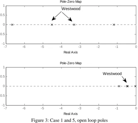
Figure 3: Case 1 and 5, open loop poles
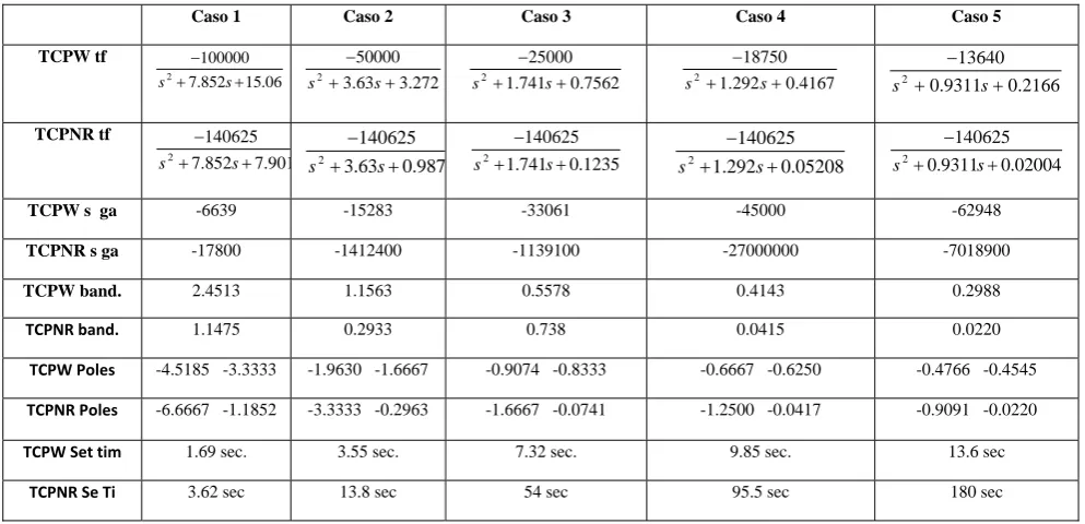
Table II shows a comparison between TCPW and TCPNR in terms of open loop transfer function, static gain, bandwidth and poles and zeros.
As it was hinted in previous section, the span of variation of TCPW’s static gain is smaller than the one of TCPNR. In fact, the standard deviation of TCPW static gain is 2.3104 and TCPNR standard deviation is 2.9106. If a controller is tuned for a certain network parameters and then there are changes, TCPW will perform much better.
Looking at the last two rows of Table II and Figure 3, we can see that the open loop poles of TCPW lie between the poles of TCPNR. Moreover, the greater the delay, the closer the poles to the origin, i.e., the slower the system.
Figure 4: Open loop step responses and settling times
Figure 4 shows the open loop step response of both TCP variants considering the delay. Settling times are smaller for TCPW (as shown in Table II). The greater the delay is, the slower the system and greater the gain are. Clearly, TCPNR is slower than TCPW.
[image:5.595.316.542.74.456.2]Figures 5 and 6 depict the open loop magnitude Bode diagram of each system. Again, TCPNR has a worst behavior than TCPW. TCPW’s bandwidth is bigger than TCPNR’s one: Westwood is more robust when there are
Figure 5: Open loop TCPW Magnitude Bode plot
10-3 10-2 10-1 100 101 102 103
0 20 40 60 80 100 120 140
Mag
ni
tud
e (
dB
)
Open loop BODE New reno
Frequency (rad/sec)
[image:5.595.51.270.452.632.2]0.15 0.3 0.6 0.8 1.1
Figure 6: Open loop TCPNR Bode diagram
A. Second experiment: Changing N, fixed R
The second experiment considers a fixed R and a changing number of users:
TABLEIII NETWORK CONFIGURATIONS
N R C P0 Q
Case1 40 0.3 3750 0.0025 200 Case2 50 0.3 3750 0.0040 200 Case3 70 0.3 3750 0.0077 200 Case4 100 0.3 3750 0.0158 200 Case5 2000 0.3 3750 0.0632 200
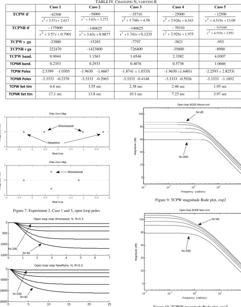
Observing Table IV, it can be concluded that the bigger N give smaller the static gain. Again the standard deviation of the static gain is smaller for TCPW (9284) than for TCPNR (86497). Moreover, the bandwidth increases with the number of users.
As in experiment 1, all the poles are stable (Table IV and Figure 7). In fact, TCPW’s poles are always placed between TCPNR’s poles. As R is constant, the farthest pole is located at -1/R.
0 2 4 6 8 10 12 14 16 18 20
-4000 -3000 -2000 -1000 0
Open loop step Westwood, N=50, R
0 50 100 150 200 250 300 350
-4 -3 -2 -1
0x 10
5 Open loop step NewReno, N=50, R
0.3
0.6 0.8 1.1 0.15
0.15, 0.3 0.6
0.8 1.1
10-3 10-2 10-1 100 101 102 103
0 20 40 60 80 100 120 140
M
agn
itude (
dB
)
Open loop BODE Westw ood
Frequency (rad/sec)
0.15 0.3 0.6
0.8 1.1
-7 -6 -5 -4 -3 -2 -1 0
-1 -0.5 0 0.5 1
Pole-Zero Map
Real Axis
-7 -6 -5 -4 -3 -2 -1 0
-1 -0.5 0 0.5 1
Pole-Zero Map
Real Axis
Westwood
TABLEIV.CHANGING N, VARYING R
Caso 1 Caso 2 Caso 3 Caso 4 Caso 5
TCPW tf
617 2 57 3
62500 2
. s .
s
272 . 3 63 . 3
50000
2
s
s 3748 458
35710 2 . s .
s
543 6 926 3
25000 2 . s .
s
09 13 519 4
12500
2 . s .
s
TCPNR tf
7901 0 57 3
175800 2 . s .
s
9877 . 0 63 . 3
140625
2
s
s 1.741 0.1235 140625
2
s
s 3926 1975 70310 2 . s .
s
951 3 519 4
315160
2 . s .
s
TCPW s ga -23880 -15283 -7797 -3821 -955
TCPNR s ga 222470 -1423800 -726400 -35600 -8900
TCPW band. 0.9044 1.1563 1.6546 2.3382 4.0307
TCPNR band. 0.2353 0.2933 0.4076 0.5738 1.0666
TCPW Poles -2.5399 -1.0305 -1.9630 -1.6667 -1.8741 ± 1.0335i -1.9630 ±1.6401i -2.2593 ± 2.8253i
TCPNR Poles -3.3333 -0.2370 -3.3333 -0.2963 -3.3333 -0.4148 -3.3333 -0.5926 -3.3333 -1.1852
TCPW Set tim 4.6 sec 3.55 sec 2.38 sec 2.46 sec 1.95 sec
TCPNR Set tim 17.1 sec 13.8 sec 10.1 sec 7.23 sec 3.97 sec
-4 -3.5 -3 -2.5 -2 -1.5 -1 -0.5 0
-5 0 5
Pole-Zero Map
Real Axis
Ima
g
ina
ry
A
x
is
-4 -3.5 -3 -2.5 -2 -1.5 -1 -0.5 0
-5 0 5
Pole-Zero Map
Real Axis
Ima
g
ina
ry
A
x
is
Westwood
Newreno
[image:6.595.50.533.52.667.2]Westwood
Figure 7: Experiment 2. Case 1 and 5, open loop poles
0 1 2 3 4 5 6 7
-1500 -1000 -500 0
Open loop step Westwood, N, R=0.3
0 5 10 15 20 25
15000 10000 -5000 0
Open loop step NewReno, N, R=0.3 N=40
N=200
N=40 N=200
Figure 8: Experiment 2: Open loop step responses and settling times The settling times (Figure 8, Table IV) are not so different as in experiment 1. Again TCPW is faster than TCPNR and the settling times are more similar. The
magnitude Bode diagrams (Figures 9 and 10) are more similar than in experiment 1.
10-2 10-1 100 101 102
0 20 40 60 80 100
Ma
gni
tud
e (
d
B
)
Open loop BODE Westw ood
Frequency (rad/sec)
[image:6.595.318.543.469.653.2]N=200 N=40
Figure 9: TCPW magnitude Bode plot, exp2
10-2 10-1 100 101 102
0 20 40 60 80 100
M
agni
tude (
d
B
)
Open loop BODE New reno
Frequency (rad/sec)
N=40
N=200
Figure 10: TCPNR magnitude Bode plot, exp2
A. Third experiment: Mixed situations
[image:6.595.50.270.479.671.2]TABLEV NETWORK CONFIGURATIONS
N R C P0 Q
Case1 80 0.1 3750 0.0910 200 Case2 40 0.9 3750 0.0003 200 Case3 60 0.25 3750 0.0082 200 Case4 50 0.3 3750 0.0040 200
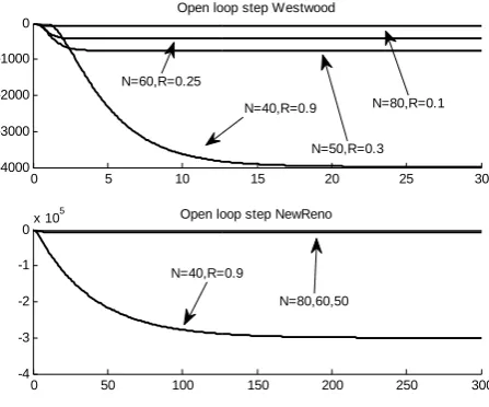
The open loop step responses are shown in Figure 11. The trends and comments regarding static gain, bandwidth and poles follow those given for experiments 1 and 2. It can be seen that the bigger the delay, the bigger the gain is. In fact, when the delay is big, TCPNR is clearly slower than TCPW (Figure 11).
0 5 10 15 20 25 30
-4000 -3000 -2000 -1000 0
Open loop step Westwood
0 50 100 150 200 250 300
-4 -3 -2 -1
0x 10
5 Open loop step NewReno
N=40,R=0.9 N=50,R=0.3 N=60,R=0.25
N=80,R=0.1
N=40,R=0.9
[image:7.595.328.555.51.238.2]N=80,60,50
Figure 11: TCPW and TCPNR open loop step response Case 4 is the working scenario: 50 users and a delay of 0.3 seconds. Using the classical method of Ziegler-Nichols [8] followed by some fine tuning, two controllers were tuned, one for TCPW and the other for TCPNR.:
TCPW: Kp= -0.000015, Ti=5, Td=0.
TCPNR: Kp= -0.00002, Ti=3, Td=0.05
[image:7.595.57.276.53.123.2]The TCPW controller is a PI, the derivative term has been set to zero because there was no improvement when including this term.
Figure 12 shows the closed loop response of the TCPW system for the 4 scenarios under study. It represents the evolution of the router’s queue (controlled variable) when a step is applied. Figure 13 shows the control variable (probability): how it changes to drive the queue to the desired value.
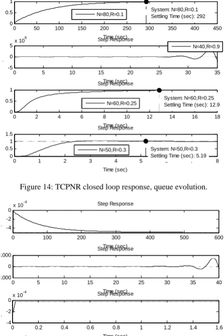
Figures 13 and 14 depict the closed loop behavior of the TCPNR system for the four scenarios under study. The controlled variable (queue size at the router) corresponds to Figure 12 (best settling time 18.2 sec., case 2 and the worst time is 867 sec. in Case1) and the probability of marking a packet is showed in Figure 13.
0 200 400 600 800 1000 1200
0 0.1 0.2 0.3 0.4 0.5 0.6 0.7 0.8 0.9 1
Closed loop response. Westw ood
Time (sec)
A
m
pl
itude
[image:7.595.317.546.70.451.2]N=80,R=0.1 N=60,R=0.25 N=50,R=0.3 N=80,R=0.1
Figure 12: TCPW closed loop response, queue evolution.
0 200 400 600 800 1000 1200 1400 1600 1800 -7
-6 -5 -4 -3 -2 -1 0 1x 10
-4 Closed loop response. PROBABILITY. Westw ood
Time (sec)
A
m
pl
itude
N=80,R=0.1
N=60,R=0.25 N=50,R=0.3 N=40,R=0.9
Figure 13: TCPW closed loop response, probability
Observing Figures 12 and 13, we can conclude that the step response is stable in all cases. When N and R are closer to the nominal scenario, the results are better. But what it is really important is that the system is robust to changes in the parameters. Looking at Figures 14 and 15 some conclusions are similar: the most similar the scenario to the nominal one (fourth graph) the better the results.
[image:7.595.49.273.226.412.2] [image:7.595.315.539.259.449.2]Step Response
Time (sec)
0 5 10 15 20 25 30 35
-5 0 5x 10
6 Step Response
Time (sec)
p
Step Response
Time (sec) Step Response
Time (sec)
0 50 100 150 200 250 300 350 400 450
0 0.5 1
System: N=80,R=0.1 Settling Time (sec): 292
0 2 4 6 8 10 12 14 16 18
0 0.5 1
System: N=60,R=0.25 Settling Time (sec): 12.9
0 1 2 3 4 5 6 7 8
0 0.5 1 1.5
System: N=50,R=0.3 Settling Time (sec): 5.19 N=80,R=0.1
N=40,R=0.9
N=60,R=0.25
[image:8.595.50.273.61.395.2]N=50,R=0.3
Figure 14: TCPNR closed loop response, queue evolution.
0 100 200 300 400 500 600
-4 -2 0
x 10-4 Step Response
Time (sec)
p
0 5 10 15 20 25 30 35 40
1000 0 1000
Step Response
Time (sec)
0 0.2 0.4 0.6 0.8 1 1.2 1.4 1.6
-4 -2
0x 10
-4 Step Response
Time (sec)
p
0 0.5 1 1.5 2 2.5 3 3.5 4
-4 -2
0x 10
-4 Closed loop response. PROBABILITY. New Reno
Time (sec)
[image:8.595.51.271.243.441.2]p
Figure 15: TCPNR closed loop response, probability
VI. CONCLUSION
The paper has presented a detailed analysis of TCP Westwood and TCP NewReno in terms of poles, static gain and frequency response of its linearized transfer functions, parametrized in terms of the network parameters. This has made possible to compared their expected responses for the same traffic conditions: The main conclusion is that as variations in the static gain and bandwidth are smaller for TCP Westwood and its bandwidth is bigger, the controlled system will be more robust in the inherent presence of changes in the network parameters: it has been shown that it can work properly in a wide range of situations as it has been shown through examples. Moreover, the TCP Westwood transfer function model has damping greater than 0.8.
Results are encouraging and more work is being done to use this information, such as using techniques for tuning the controller that takes into account the expected parameter variations.
ACKNOWLEDGMENT
The authors would like to thank Prof. F. Tadeo for so many fruitful discussions.
REFERENCES
[1] Azuma, T., T. Fujita, M. Fujita (2006). Congestion control for TCP/AQM networks using State Predictive Control. Electrical Engineering in Japan, 156, 1491-1496.
[2] Aström K.J. and T. Hägglund (2006), Advanced PID control. ISA. NC.
[3] Deng, X., S. Yi, G. Kesidis. C.R. Das (2003). A control theoretic approach for designing adaptive AQM schemes. GLOBECOM’03, 5, 2947 – 2951.
[4] Jacobson, V. (1988). Congestion avoidance and control. ACM SIGCOMM’88.
[5] Ryu, S., C. Rump, C. Qiao (2004). Advances in Active Queue Management (AQM) based TCP congestion control. Telecommunication Systems, 25, 317-351.
[6] Floyd, S., & Jacobson, V. (1993). Random early detection gateways for congestion avoidance. Networking, IEEE/ACM Transactions on, 1(4), 397-413.
[7] Mathis, M., Semke, J., Mahdavi, J., & Ott, T. (1997). The macroscopic behavior of the TCP congestion avoidance algorithm. ACM SIGCOMM Computer Communication Review, 27(3), 67-82.
[8] Dorf, R. C. (1995). Modern control systems. Addison-Wesley Longman Publishing Co., Inc.
[9] Franklin, G. F., Powell, J. D., & Emami-Naeini, A. (1994). Feedback control of dynamics systems. Addison-Wesley, Reading, MA.
[10] Hollot, C.V., V. Misra, D. Towsley, W. Gong (2002). Analysis and Design of Controllers for AQM Routers Supporting TCP flows. IEEE Transactions on Automatic Control, 47, 945-959. [11] Bolajraf, M., Tadeo, F., Alvarez, T., & Rami, M. A. (2010).
State-feedback with memory for controlled positivity with application to congestion control. IET control theory & applications, 4(10), 2041-2048.
[12] Hohenbichler, N. (2009). All stabilizing PID controllers for time delay systems. Automatica, 45, 2678-2684.
[13] Silva, G., A. Datta and S. Bhattacharyya. PID controllers for time-delay systems. Birkhäuser, 2005.
[14] Long, G.E., B. Fang, J.S. Sun and Z.Q. Wang (2010). Novel Graphical Approach to Analyze the Stability of TCP/AQM Networks. Acta Automatica Sinica, 36, 314-321.
[15] Teresa Alvarez, Diego Martínez (2013), Handling the Congestion Control Problem of TCP/AQM Wireless Networks with PID Controllers, in IAENG Transactions on Engineering Technologies, pages 365-379.
[16] M. di Bernardo, L. A. Grieco, S. Manfredi, and S. Mascolo," Design of robust AQM controllers for improved TCP Westwood congestion control", Proc. of the 16th International Symposium on Mathematical Theory of Networks and Systems (MTNS 2004), Katholieke Universiteit Leuven, Belgium, July, 2004.
[17] Chen, J., F. Paganini, M.Y. Sanadidi, R. Wang and M. Gerla (2006). Fluid-flow analysis of TCP Westwood with RED. Computer Networks, 50, 132-1326.
[18] Mascolo, S., C. Casetti, M. Gerla, M.Y. Sanadidi, R. Wang. TCP Westwood: bandwidth estimation for enhanced transport over wireless links, in: Proceedings of Mobicom, 2001.
[19] Hollot, C.V. and Y. Chait (2001). Nonlinear stability analysis for a class of TCP/AQM networks”. In Proceedings of the 40th IEEE Conference on Decision and Control, Orlando, USA.
[20] Al-Hammouri, A.T., V. Liberatore, M.S. Branicky, and S.M. Phillips (2006b). Parameterizing PI congestion controllers. Proc. First International Workshop on Feedback Control Implementation and Design in Computing Systems and Networks, Vancouver, CANADA.