Abstract—A validated simulation model primarily requires performing an appropriate input analysis mainly by determining the behavior of real-world processes using probability distributions. In many practical cases, probability distributions of the random inputs vary over time in such a way that the functional forms of the distributions and/or their parameters depend on time. This paper answers the question whether a sequence of observations from a process follows the same statistical distribution, and if not, where the exact change points are. We propose a Likelihood Ratio Test (LRT) based method to detect multiple change points when observations follow non-stationary Poisson process with diverse occurrence rates over time. Results from a comprehensive Monte Carlo study indicate satisfactory performance for the proposed methods.
Index Terms—Simulation input data analysis, Non-stationary Poisson process, Cluster analysis, Change point detection.
I. INTRODUCTION
IMULATION input data analysis is often considered as a vital step in most simulation experiments enabling analysts to drive reasonable models from real world systems. The ultimate goal of input data analysis is selection of valid input models, mainly the statistical distributions that appropriately represent the behavior of the system under consideration. In the simplest case, an input parameter is assumed to be independent and identical random variable (i.i.d), which follows a known and standard distribution. However, in many real-world cases, there is no guarantee that such assumptions are always met. [1] Noted that there are many alternatives to these assumptions that can be addressed in different applications. For instance, the input data may be correlated which means the consecutive observations depend on each other. In fact, the observation t can be modeled with a linear or nonlinear combination of the last observations t − 1, t − 2, . . . together with an independent white noise.
A general model frequently used to represent non-stationary processes, especially arrival times, is Nonhomogeneous Poisson Processes (NHPP), which has
Issac Shams is with the Department of Industrial and Systems Engineering, Wayne State University, Detroit, MI, 48202 USA. (e-mail: [email protected]).
Saeede Ajorlou, is with the Department of Industrial and Systems Engineering, Wayne State University, Detroit, MI, 48202 USA. (e-mail: [email protected]).
Kai Yang, is with the Department of Industrial and Systems Engineering, Wayne State University, Detroit, MI, 48202 USA. (e-mail: [email protected]).
successfully been performed to model complex time-dependent arrival processes in many simulation studies [2]. In a NHPP, it is assumed that the arrival rate λ depends on time. Hence, N(t), the number of arrivals during the time interval (0,t], varies over time and time-dependent arrival rate denoted by λ(t) is a nonnegative, integral function satisfying the usual Poisson assumptions.
In case that the arrival rate exhibits a strong dependence or a specific and complex pattern i.e. cyclic, nested cyclic, or trend patterns, researchers often estimate the mean-value function E[N(t)] over time using different parametric and nonparametric methods. [3], [4], and [5] addressed the estimation of mean- value function using parametric methods. [6], [7], [8], [9], [10], [11], [12], [14], and [13] proposed different nonparametric or semi-parametric methods to estimate the mean-value of a NHPP as a function of t. Alternatively, another method used to model such a process is to divide the time interval (0, t] to a finite number of disjoint subintervals and estimate λi for the ith subinterval.
[15] Discussed that this method is a heuristic but practical approach; however, there is still an important unanswered question on how one decides on the length of subintervals. Although a graphical method for approximately determination of the subinterval bounds is proposed, but the performance of the suggested method is not investigated through the use of statistical measures. In this paper, we propose an approach, based on LRT, capable of detecting the cluster patterns in a given data set and estimating the change points (the subintervals of length) for each cluster. We examine our proposed method using a comprehensive simulation study and different performance measures, i.e. change point locations and dispersions and number of detected changes. The rest of this paper is organized as follows. In Section II, the problem is discussed in details and a basis for applying change point detection techniques in simulation input analysis is provided. The LRT method is briefly presented in Section III. In Section IV, the performance of the proposed method based on accuracy and precision measures are evaluated. Lastly, our concluding remarks are presented in the final section.
II. PROBLEM STATEMENT
Change point detection techniques have successfully been used in numerous statistical methods including regression analysis, statistical process control, signal processing, and pattern recognition. These techniques typically deal with identifying the time that a change occurs in the observations of a data set collected over time. If a data set has one or more change points, at least a part of observations has different moment(s) and/or different distribution(s) from the rest of observations. In this section, we present the general problem
On Modeling Non-homogeneous Poisson
Process for Stochastic Simulation Input
Analysis
Issac Shams, Saeede Ajorlou, Kai Yang
of change point detection for simulation input variables when observations are clustered. A random input variable can be considered as a stochastic process, so data set S can be defined as a collection of random variables S={Xt; 1,2,…,m}
over time. Note that the index t represents the order of variables (discrete event variables) and S is a finite set. In order to fit a specific probability distribution to data set S, we must check whether the observations are independent and identical. The second assumption indicates that xt’s should
follow the same probability distribution ⋅ ⋅ ; 1, … , .
Now assume that xt’s are not identical but they are
clustered in R+1 different populations. In this situation, data set S can be divided into R+1 disjoint subgroups, S1,
S2…SR+1 whose union is S. Besides, it is assumed that
observations within Si are independent and identically
distributed; however, observations from two successive sets are unlike. Let τj be the jth change point in data set S where τ
j
; j=1,2,…,R is subjected to 0 < τ1 < …< τR < m. In this paper,
it is assumed that τj is the location of the first element of set
Sj, it is of interest to estimate locations of change points τj′s
in a statistical array of data obtained (or being augmented) as a result of some industrial, simulation, or other types of exper- iments. Several approaches have been proposed for the case when there are multiple changes in the location parameters of random variables. Some researchers studied nonparametric change point detection methods which do not require any distributional assumptions (See for example [20],[16] and [17]. Using single change point detection methods is another approach that can be used for the identification of multiple change points. [18] pointed out that a method for detecting and estimating a single change point may be able to apply for multiple changes by binary segmentation. Regarding this issue [19] stated that for the data sets which need not to follow any single pattern or regime, the presence of multiple change point estimators may be inaccurate. In the next section, we present a binary segmentation method, which is based on the likelihood ratio test for exponential random variables.
III. PROPOSED METHOD
Likelihood Ratio Test (LRT) has been considered as one of the most powerful tools for detecting one or more changes in a set of observations in applied statistics literature. This procedure consists of calculation of the likelihood function for all possible partitions of the data set into typically two groups. When LRT statistic exceeds a threshold value, a change point is detected and the most likely location of the change is determined by the partition corresponding to the maximum value of the statistic. The LRT method can be applied to detect not only the presence of multiple change points in an input data set, but also their locations as well. As previously stated, once a single change point is detected, the data set is divided at the estimated change point and the LRT statistic is formed separately for the two new groups. Although most researchers asserted that LRT method outperforms many competing approaches in identifying change points but it has a restrictive assumption, i.e. knowing the exact the probability distribution of the random inputs before estimating the change points. Since LRT method relies upon distributional assumptions, the probability distribution of the input data set should be specified prior to constructing an appropriate LRT statistic. Despite the fact that the probability distribution of some
input variables like interarrival time can be guessed (Law, 2007), in most practical cases, it is actually not easy to have an accurate insight about the exact distribution of the input data. In this situation, one can apply generalized likelihood ratio test derived from a general distribution such as exponential family distributions, Johnson’s system of distributions, Bzier distribution family. In this paper, we consider the case that observations simply come from an independent univariate exponential distribution with rate parameter of λ. Again assume that there is a random data set from an input variable including m independent observations x′ts such that ∼ ⋅ , ;
1, … , 1 where τj is the jth change point, τ0 =0 and τR+1
=m. Suppose that the first change point in the mean of observations which may be detected is located in the m1th observation such that m1 < m and m1 + m2 = m. Log of
likelihood function for xt is
log
e
x
t (1) and log of likelihood function for the first m1 observations islog log 1 . 1 1 1 1
1
m
t t e
eL m λ λ x (2)
This term is maximized when 1
x1 m1
xt
t1
m1
(3)
which is the maximum likelihood estimator (MLE) for the first m1 observations. The maximized value of the LRT
statistic is then
. ) (
log 1
1 1 1
1 1 m
x m m
L m
t t
e
(4)
Similarly, the likelihood function for the remaining m2
=m-m1 observations is maximized when
m
m m t
t
x m x
1 2
2
1
1 (5)
with a value of
. ) (
log 2
1 2 2
2
1 m x m m
L m
m m t
t
e
(6)
Hence, under the alternative hypothesis Ha which state
that there is at least a change point in the random input data set, the maximum log-likelihood function for all observations is the sum of the two log-likelihood functions
Conversely, if all m observations in the input data set are independently and identically distributed then the likelihood function is maximized when
m
t t
x m x
1
1 (8)
with a value of
. ) ( log
1
0 m
x m m L m
t t
e
(9)
If La is considerably larger than L0 we could conclude Ha
with 100 (1-) percent, i.e. our input data are not homogeneous over the whole time span in which they were being gathered. This enables us to statistically diagnose the presence of nonhomogeneity in random input data set S={Xt;
1,2,…,m} and also provides a base for estimating the exact length of subintervals more accurately. It should be pointed out that
1 2
1 2 0
1 1 2 2
1 2
lrt , 2
2 log log log
2log
a
e e e
m m
e
m m L L
m x m x m x
x x
x x
(10)
has asymptotically a chi square distribution with one degree of freedom, with large values signaling nonhomogeneous input data. For the large sample approximation see Wilks (1947, p. 151) or Mood, Graybill, and Boes (1974, p. 441). Clearly, the value of m1, the number of observations in the
first group, which maximizes equation (13) is the maximum likelihood estimate for the change point location, provided that one exists. Hence, maximum value of equation (13) beyond a predefined boundary indicates that input observations are not all from an identical distribution.
At this point, we shall consider the behavior of the statistic in equation (13) briefly. Based on 4000 simulation runs each with m observations derived from a homogeneous exponential distribution, Elrt [m1,m2], the estimated
expected value of equation (13) is calculated for each value of m1 using
Elrt
m m1, 2
Elrt
m m1, 2
. (11) Without loss of generality, it is assumed that m is 50 and the homogeneous distribution has a mean equal to 1/λ. The results (not reported here) imply that the homogeneous expected value of equation (13) is not the same for all values of m1. If m1 or m2 is small, the expected value is alwayslarger than when they get close to each other. In fact, expected value of likelihood ratio tests is likely to be shaped as a bathtub with heavy tails. Therefore, it is desirable to improve the statistic in (13) by dividing each statistic by its relevant homogeneous expected value, i.e.
1 2
*
1 2
lrt , . Elrt ,
m m lrt
m m
(12)
In this way the resulting expected value is the same for all values of m1. So we apply the improved test statistic in
(15) instead of equation (13) in our study. In the next section, we statistically compare the efficacy of our proposed methods using Monte Carlo simulation.
IV. NUMERICAL EXAMPLES
Researchers often use two different categories of measures for comparing the efficiency of change point detection techniques namely accuracy performance that shows how close a measured value is to the actual value and precision performance that rates how close the measured values are to each other. To completely investigate the performance of the proposed change point estimator, we report measures evaluating both categories for the case that there are multiple changes in random input data S. It is assumed that input observations are univariate exponential random variables and there are R changes in the data set. The rate parameter in each group is identical but they differ between consecutive groups. Presume Λ={μj+1| μj+1 = μj + δ×(-1)j;
μj=1/λj; j=0,1,…,R-1} is the set of change values where λ0 is
a predefined initial value and δ is the magnitude of change.
Λ is defined such that the difference in rate parameter for two consecutive groups is identical and equal to δ. For example, imagine that there are R=4 groups with different rate parameter values and let λ0 = 1 and δ = 3. In this case,
sequence Λ is defined as Λ = {1, 4, 1, 4}. We also consider equally spaced changes alternating between two groups. For example, a single change would be midway in the data sets, and two shifts would be after one-third and two-third of the data sets, etc. One could consider an alternative model in which the change locations would be specified randomly (Turner (2001)).
A. Accuracy performances of change point estimator
It is assumed that there are m=200 observations from a simulation input variable and it is of interest to detect any changes in random data set S and their locations. The number of changes are set equal to R=1, 2, 3, 4 and τj;
j=1,…,R is the true location of the jth change. Thus, if there
is a single change in the data set, then R=1, τ1 = 101 and
there are two different groups. The first group consists of the first 100 observations and the second group consists of the second 100 observations. Similarly, if there are four changes in the data set, R=4 then τ1 to τ4 are namely 40, 80, 120, and
160. In this case, there are five different groups: the first group consisting of the first observation to the 40th
observation, the second group consisting of the 41st
observation to the 80th observations and so on. To estimate
τj’s, 1000 replications are used in each simulation run. Both
change point estimators can be designed to be capable of detecting at most seven potential changes. However, one could design both change point detection techniques to be capable of detecting and estimating more or less changes. Considering at most seven changes in a data set of size 200, we can evaluate the first seven dj*’s in clustering method
For the clustering method, the threshold values for d1* to
d7* are set equal to 0.7686, 0.9435, 0.7571, 0.8119, 0.7343,
0.7369 and 0.6911, respectively leading to probability of false detection values (type I error) namely 0.03, 0.02, 0.02 0.01, 0.01, 0.01, and 0.01. In this case, according to Bonferroni inequality, the overall probability of false detection (overall) cannot exceed 0.11. The threshold values
were calculated via Mont Carlo simulation by generating 100 sets each consisting of 100 values of d1* to d7* and
estimating the 100(1- α) percentiles of d1* to d7* where
there is no change in the data sets. It is also worth mentioning, we apply the Box-Cox transformation for xt’s as
shown in equation (3) to stabilize the standard deviation of input variables and increase the performance of the clustering method. Using 100,000 observations, η was estimated to be 0.24. Therefore, all observations transform into x0.24. Also we take into account the effects that may
caused by not using the Box-Cox transformation and also by using top-down (divisive) hierarchical clustering algorithm instead of bottom-up method.
Also for the LRT method, we first estimate Elrt array for all possible values of m1 using 4,000 simulation runs while
m=200 and then we utilize the improved statistic in equation (15). If lrt1* exceeds its corresponding threshold value, the
data are separated at the location of lrt1*. Then the method
is repeated for two new subsets and is continued for at most 20+21+22=7 segments. The threshold values for lrt
1* to lrt7*
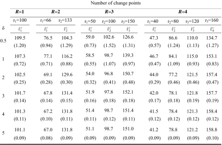
are set equal to 0.7686, 0.9435, 0.7571, 0.8119, 0.7343, 0.7369, and 0.6911, respectively leading to probability of false detection values (type I error) namely 0.03, 0.02, 0.02 0.01, 0.01, 0.01, and 0.01. Table 1 shows the estimate of change point(s) obtained by clustering method and their standard errors (in the parenthesis) where there are R=1, 2,
3, and 4 changes in the simulation input data. As mentioned before, we investigate the seven consecutive dj’s
and select the last jth which exceeds its threshold value. If d
q;
q < 7, is the last dj’s that is greater than its threshold value,
Then lj; j=1,2,…,q is considered as the estimate of the jth
change point location. Because there are R changes in the input data set, the value of q > R indicates one or more false detections.
In Table 1, we consider the R first change point locations lj’s, where q > R and the q first change point locations where
q< R. It can be observed that the hierarchical clustering method performs properly when the magnitude of change in the mean is greater than 1 (δ>1). For small changes in the mean value, the clustering method has a bias, which increases as the magnitude of change decreases.
However, for larger magnitude of changes in rate parameter (δ>1), the estimates of change locations are approximately unbiased. It is worth mentioning that hierarchical clustering method tends to overestimate the locations of the first changes and underestimate the locations of the last changes. Table 2 displays the estimates of change locations based on the LRT method with their related standard error (in the parenthesis) when there are R+1 subgroups differing in rate parameter. Note that the LRT method performs effectively when there is a single change point in the input data set and provides unbiased estimates for change location.
This method performs appropriately as well if there are more than one changes and the magnitude of shift is larger than one. Although there is a small biasness, particularly in intermediate change points, the magnitude of biasness is not very large to seriously affect groups.
Number of change points
R=1 R=2 R=3 R=4
τ1=100 τ1=66 τ2=133 τ1=50 τ2=100 τ3=150 τ1=40 τ2=80 τ3=120 τ3=160
δ τc
1
ˆ τc
1
ˆ τc
2
ˆ τc
1
ˆ τc
2
ˆ τc
3
ˆ τc
1
ˆ τc
2
ˆ τc
3
ˆ τc
4
ˆ
0.5 109.5 76.5 104.3 59.0 102.6 126.6 47.3 86.6 110.0 134.7
(1.20) (0.94) (1.29) (0.73) (1.52) (1.31) (0.57) (1.24) (1.13) (1.27)
1 107.3 77.1 116.2 58.5 98.7 139.3 46.7 84.1 115.0 153.1
(0.72) (0.71) (0.88) (0.55) (1.07) (0.97) (0.47) (1.09) (0.93) (0.83)
2 102.5 69.1 129.6 54.0 96.8 150.7 44.0 77.2 121.5 157.4
(0.25) (0.28) (0.30) (0.32) (0.41) (0.48) (0.29) (0.46) (0.46) (0.47)
3 101.7 67.8 131.4 51.9 97.8 152.1 42.0 78.1 121.8 157.7
(0.14) (0.14) (0.15) (0.16) (0.18) (0.18) (0.17) (0.18) (0.19) (0.19)
4 101.3 67.2 131.8 51.4 98.7 151.4 41.5 78.4 121.3 158.4
(0.11) (0.10) (0.11) (0.11) (0.12) (0.11) (0.12) (0.12) (0.12) (0.12)
5 101.1 67.0 131.8 51.1 98.7 151.0 41.2 78.8 121.2 158.8
[image:4.595.77.527.497.790.2]B. Precision performances of change point estimator
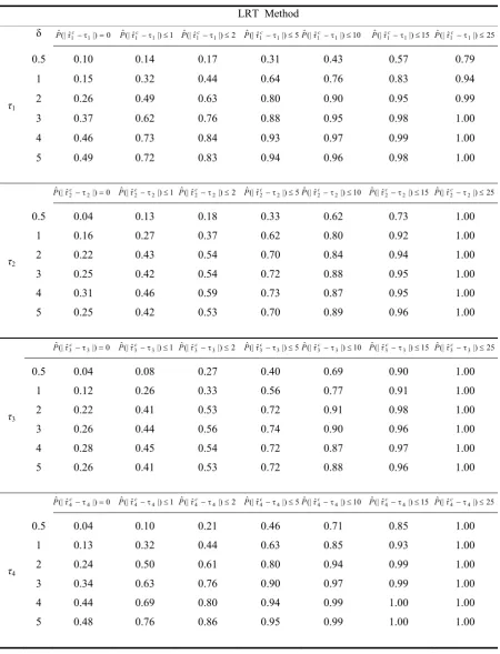
Researchers believe an esestimator with good per- formances in estimating location of changes may inherently have poor performances in terms of dispersion. In this situation, the estimator provides estimates that are close to the true location in average but far from each other. An
indication of the precision of two estimators is confidence set that is the observed frequency with which the change point estimators were within a given number of subgroups of the actual change point. Table 2 presents the precision performance values given by the LRT method over different values of δ. It is shown that although a change of size δ=0.5 may be far from the true location of change, the method totally have an appropriate performance.
LRT Method
δ Pˆ(|ˆτ1c1|)0 Pˆ(|τˆ1c1|)1 Pˆ(|τˆ1c1|)2 Pˆ(|τˆ1c1|)5Pˆ(|τˆ1c1|)10 Pˆ(|τˆ1c1|)15 Pˆ(|τˆ1c1|)25
τ1
0.5 0.10 0.14 0.17 0.31 0.43 0.57 0.79
1 0.15 0.32 0.44 0.64 0.76 0.83 0.94
2 0.26 0.49 0.63 0.80 0.90 0.95 0.99
3 0.37 0.62 0.76 0.88 0.95 0.98 1.00
4 0.46 0.73 0.84 0.93 0.97 0.99 1.00
5 0.49 0.72 0.83 0.94 0.96 0.98 1.00
0 |) ˆ (| ˆ
2 2c
τ
P Pˆ(|τˆ2c2|)1 Pˆ(|τˆ2c2|)2 Pˆ(|τˆ2c2|)5Pˆ(|τˆ2c2|)10 Pˆ(|τˆc22|)15 Pˆ(|ˆτ2c2|)25
τ2
0.5 0.04 0.13 0.18 0.33 0.62 0.73 1.00
1 0.16 0.27 0.37 0.62 0.80 0.92 1.00
2 0.22 0.43 0.54 0.70 0.84 0.94 1.00
3 0.25 0.42 0.54 0.72 0.88 0.95 1.00
4 0.31 0.46 0.59 0.73 0.87 0.95 1.00
5 0.25 0.42 0.53 0.70 0.89 0.96 1.00
0 |) ˆ (| ˆ
3 3c
τ
P Pˆ(|τˆ3c3|)1 ˆ(|ˆ |) 2
3 3c
τ
P Pˆ(|τˆ3c3|)5ˆ(|ˆ |) 10
3 3c
τ
P Pˆ(|τˆ3c3|)15 ˆ(|ˆ |) 25
3 3c
τ P
τ3
0.5 0.04 0.08 0.27 0.40 0.69 0.90 1.00
1 0.12 0.26 0.33 0.56 0.77 0.91 1.00
2 0.22 0.41 0.53 0.72 0.91 0.98 1.00
3 0.26 0.44 0.56 0.74 0.90 0.96 1.00
4 0.28 0.45 0.54 0.72 0.87 0.97 1.00
5 0.26 0.41 0.53 0.72 0.88 0.96 1.00
0 |) ˆ (| ˆ
4 4c
τ
P Pˆ(|τˆ4c4|)1 ˆ(|ˆ |) 2
4 4c
τ
P Pˆ(|τˆ4c4|)5ˆ(|ˆ |) 10
4 4c
τ
P Pˆ(|τˆ4c4|)15 ˆ(|ˆ |) 25
4 4
c
τ P
τ4
0.5 0.04 0.10 0.21 0.46 0.71 0.85 1.00
1 0.13 0.32 0.44 0.63 0.85 0.93 1.00
2 0.24 0.50 0.61 0.80 0.94 0.99 1.00
3 0.34 0.63 0.76 0.90 0.97 0.99 1.00
4 0.44 0.69 0.80 0.94 0.99 1.00 1.00
[image:5.595.74.525.89.679.2]5 0.48 0.76 0.86 0.95 0.99 1.00 1.00
V. CONCLUSION
In this paper, we address a frequently occurring problem in simulation input modeling where input data is not stable over time but can be clustered in identical groups. The methods deal with identifying the locations (groups) in such a way that the observations within each group follow the same probability distribution but observations in two consecutive groups have different distributions. Regardless the fact that our method reveals acceptable results in terms of accuracy and precision performances, it still relies on relatively tight distributional assumptions. Modifications of such obstacles can be considered as a good future research. Furthermore, the LRT method can be generalized by obtaining the LRT statistic for more general distributions i.e. Johnson distribution or exponential family distributions.
REFERENCES
[1] S. Vincent,”Handbook of Simulation; Chp. Input data analysis”, New Jersey: John Wiley and Sons, 1998.
[2] I. Shams and K. Shahanaghi “Analysis of Nonhomogeneous Input Data Using Likelihood Ratio Test,” in Proc IEEE International Conference on Industrial Engineering and Engineering Management (IEEM), Hong Kong, 2009.
[3] I. Shams, S. Ajorlou, K. Yang, “Modeling Clustered Non-Stationary Poisson Processes for Stochastic Simulation Inputs,” Computers & Industrial Engineering, vol. 64, pp. 1074-1083, 2013.
[4] M. E. Kuhl, J. R. Wilson, M. A. Johnson, ”Estimating and simulating Poisson processes having trends or multiple periodicities”, IIE Transac- tions, vol. 29, pp. 201–211, 1997.
[5] M. E. Kuhl, J. R. Wilson, ”Least squares estimation of nonhomogeneous Poisson processes”, Journal of Statistical Computation and Simulation, vol. 67, pp. 75–108, 2000.
[6] P. A. W. Lewis, G. S. Shedler, ”Statistical analysis of non-stationary series of events in a data base system”, IBM Journal of Research and Development, vol. 20, pp. 465–482, 1976.
[7] S. Ajorlou, I. Shams, and M. G. Aryanezhad. "A Genetic Algorithm Approach for Multi-Product Multi-Machine CONWIP Production System." Applied Mechanics and Materials, vol. 110, pp. 3624-3630, 2012.
[8] L. M. Leemis, ”Nonparametric estimation of the cumulative intensity function for a nonhomogeneous Poisson process”, Management Science, vol. 37, pp. 886–900, 1991.
[9] L. M. Leemis, ”Nonparametric estimation of the cumulative intensity function for a nonhomogeneous Poisson process from overlapping re- alizations”, Management Science, vol. 46, pp. 989–998, 2000. [10] L. M. Leemis, ”Nonparametric estimation and variate generation for
a nonhomogeneous Poisson process from event count data”, IIE Transac- tions, vol. 36, pp. 1155–1160, 2004.
[11] M. E. Kuhl, J. R. Wilson, ”Modeling and simulating Poisson processes having trends or nontrigonometric cyclic effects”, European Journal of Operational Research, vol. 133, pp. 566–582, 2001. [12] M. E. Kuhl, S. G. Sumant, J. R. Wilson, ”An automated
multiresolution procedure for modeling complex arrival processes”, INFORMS Journal on Computing, vol. 18, pp. 3–18, 2006.
[13] S. Ajorlou, I. Shams “ Artificial bee colony algorithm for CONWIP production control system in a multi-product multi-machine manufacturing environment, ”Journal of Intelligent Manufacturing, vol 24, pp. 1145-1156, 2013.
[14] C. Alexopoulos, D. Goldsman, J. Fontanesi, D. Kopald, J. R. Wilson, ”Modeling patient arrival times in community clinics”, Omega, vol. 36, pp. 33–43, 2008.
[15] I. Shams, S. Ajorlou, K. Yang (2014), “A predictive analytics approach to reducing avoidable hospital readmission. arXiv preprint arXiv:1402.5991.
[16] B. E. Brodsky, B. S. Darkhovsky ”Nonparametric methods in change- point problems”, Netherland: Kluwer Academic Publishers, 1993.
[17] D. Ferger, ”Nonparametric tests for nonstandard change-point prob- lems”, The Annals of Statistics, vol. 23, pp. 1848-1861, 1995. [18]S. Ajorlou, I. Shams, K. Yang, (2014) “An analytics approach to
designing patient centered medical homes,” arXiv preprint arXiv: 1402.6666.
[19] J. H. Sullivan, ”Detection of multiple change points from clustering
individual observations”, Journal of Quality Technology, vol. 34, pp. 374– 383, 2002.
[20] E. Carlstein, ”Nonparametric change-point estimation”, The Annals of Statistics, vol. 16, pp. 188-197, 1988.
[21] S. Ajorlou, I. Shams, M. G. Aryanezhad, “Optimization of a multiproduct conwip-based manufacturing system using artificial bee colony approach” in Proc of the international multiconference of engineers and computer scientists (IMECS), Hong Kong, 2011, pp 1385-1389.
[22] A. M. Mood, F. A. Graybill, D. C. Boes, ”Introduction to the Theory of Statistics”, 3rd ed. New York: McGraw-Hill, 1974.