Extending the geological calibration of the geological time scale

University of Southampton Research Repository

ePrints Soton

Copyright © and Moral Rights for this thesis are retained by the author and/or other

copyright owners. A copy can be downloaded for personal non-commercial

research or study, without prior permission or charge. This thesis cannot be

reproduced or quoted extensively from without first obtaining permission in writing

from the copyright holder/s. The content must not be changed in any way or sold

commercially in any format or medium without the formal permission of the

copyright holders.

When referring to this work, full bibliographic details including the author, title,

awarding institution and date of the thesis must be given e.g.

AUTHOR (year of submission) "Full thesis title", University of Southampton, name

of the University School or Department, PhD Thesis, pagination

Extending the astronomical

calibration of the geological

time scale

by

Heiko P¨alike

Clare College

This dissertation is submitted for the degree of

Doctor of Philosophy

University of Cambridge

Declaration

“This dissertation is the result of my own work and includes nothing which is the outcome of work done in collaboration. It does not exceed the page limit and is not substantially the same as any work that has been, or is being sub-mitted, to any other University for any degree, diploma, or other qualification.”

Heiko P¨alike October 2001

Abstract

This thesis arises from the fact that changes in the geometry of the Earth-Sun sys-tem, due to the gravitational interaction among the planets, cause quasi-cyclic climatic variations that are imprinted in the geological record.

A speech-recognition method is adapted to provide an automated procedure to cal-ibrate cyclic geological data to astronomical calculations. Synthetic data are used to test the performance of the new method. The new algorithm is then applied to litho-logical data. Results show that the method is well suited to objectively match geolitho-logical data to astronomical calculations of the Earth’s orbit.

The calibration of the geological time scale is extended into the late Paleogene. This is achieved by generating a lithological proxy record employing an X-ray fluorescence Core Scanner that non-destructively determines elemental concentrations of calcium and iron on split sediment cores. These data exhibit cyclic variations that are shown to be of astronomical origin, and are then used to calibrate the relative duration of magne-tochrons C16 through C18. Advanced time series analysis methods are used to extract the astronomical signal. It is shown that the most recent published astronomical solu-tion is not compatible with geological data from the late Paleogene.

This new late Eocene time scale is independently confirmed by measurements of stable isotope ratios of oxygen and carbon, obtained from the same material, providing a high-resolution record of climatic variations over intervals of the late Middle and Late Eocene for the first time.

Astronomically calibrated geological data are analysed to extract parameters that are required for the calculation of detailed astronomical models. Very small changes in the precession constant of the Earth are extracted by developing a new interference method. This leads to the extraction of the long-term evolution of the tidal dissipation and dynamical ellipticity parameters of the Earth.

Geological data spanning the last∼37 million years are used to extract long term amplitude modulation patterns of the climatic signal. A comparison of the long term amplitude modulation derived from published astronomical calculations on the one hand, and those derived from a new calculation on the other hand (J. Laskar, 2001, unpublished) shows that the geological record supports the validity of the new solution. This study forms the basis for a further extension of the astronomical calibration of the geological time scale into earlier parts of the Paleogene.

Acknowledgments

Nick Shackleton has been a constant source of encouragement, enthusiasm, superb ideas, friendship, and excellent food. Without doubt working with him has been the greatest experience during my research. My parents and brother have provided sup-port in every possible way, and I could not be more grateful for their encouragement, interest and help.

Throughout my research I have been encouraged and helped by many superb characters. Jacques Laskar at the Bureau des Longitudes and Paris, and his colleagues Alexandre Correia and Benjamin Levrard, were always interested in the implications of geological research on their invaluable astronomical calculations. They helped me in many ways, and provided excellent hospitality during several trips to Paris. Marie-France Loutre at the Universit´e Catholique de Louvain taught me astronomical theory and spectral analysis during her sabbatical in Cambridge, and was very patient in answering many questions. I also thank her colleagues Michel Crucifix and Andr´e Berger.

Jerry Mitrovica and Jon Mound, at the University of Toronto, have been very interested in the implications of this research on mantle convection, and provided excellent feedback and critical comments. Jerry’s invitation to Toronto was one of the highlights during my research. Andy Gale and Ewan Laurie at the University of Greenwich introduced me to the delights of Eocene successions on the Isle of Wight, and in addition increased my knowledge of great wines, indigenous sea-food, and were always a good source of humour. Jim Zachos and Lisa Sloan gave immense encouragement, friendship, and support. Bridget Wade allowed me to work with her samples, and was great in every other way.

Didier Paillard (Gif-sur-Yvette), Andreas Prokoph (Ottowa), Athanassios Kassidas (McMaster University) and Benjamin Cramer (Rutgers) provided many software tools that proved invaluable during the course of this research.

I also thank Graham Weedon, Lucas Lourens, Ulla R¨ohl, Paul Wilson, Tjeerd van Andel, Alan Smith, Nicky White, Dan McKenzie, Paul Pearson, Isabella Raffi, Phil Saxton, Nick McCave and Harry Elderfield for advice. Simon Crowhurst provided inspiration for many things, of which computing was only one aspect. I also thank everyone else in the Department and the Godwin Laboratory, past and present.

Sam Gibbs proved to be a great friend and office partner, providing constant fun and encouragement. Other people that come to mind in no particular order are Fiona, Sam B., Paul F., Paul B., Kitty, Paul W., Steve J., Steve B., Marie, Carrie, Paula, Emily, Emilie, Tim, Hayley, Mark R., Patrizia, Lucia, Luke, Isabel C., Isabel S., John, Jon, Ben W., Chop, Henning, Angus, Martin, Jim, Alex W., Dave L., Ed, Charlie, Dan, Megan, Debs, Mike, Carine, Jemma, and without doubt many others who I inadvertently forgot. Thank you all for great fun!

Financial support was provided by the University of Cambridge, NERC studentship GT4/98/ES/50, the Cambridge Philosophical Society, Clare College, the Cambridge Eu-ropean Trust, a Royal Society-CNRS traveling grant, a Shell postgraduate bursary, and the British Chamber of Commerce in Germany. Writing this dissertation has been greatly facilitated by the use of the LA_{TEX document preparation system.}

Contents

Declaration ii

Abstract iii

Acknowledgments iv

List of Figures vii

List of Tables viii

Chapter 1 Introduction, historical overview and astronomical theory 1

1.1 Introduction . . . 1

1.2 Outline of Dissertation . . . 2

1.2.1 Chapter one outline . . . 2

1.2.2 Chapter two outline . . . 2

1.2.3 Chapter three outline . . . 2

1.2.4 Chapter four outline . . . 3

1.2.5 Chapter five outline . . . 3

1.2.6 Chapter six outline . . . 3

1.3 The age of the Earth - A historical overview . . . 4

1.4 A history of cyclostratigraphy and “Milankovitch” theory . . . 6

1.5 The development of detailed astronomically calibrated time scales . . . 9

1.6 Astronomical theory . . . 10

1.6.1 Celestial mechanics . . . 11

1.7 The origin of orbital frequencies . . . 12

1.7.1 Fundamental frequencies of the solar system . . . 13

1.7.2 General precession of the Earth . . . 14

CONTENTS vii

1.7.4 Obliquity . . . 17

1.7.5 Climatic Precession . . . 18

1.7.6 Insolation . . . 20

1.7.7 Amplitude modulation patterns: the “fingerprint” of orbital cycles 21 1.7.8 Tidal dissipation and dynamical ellipticity . . . 22

1.7.9 Chaos in the solar system . . . 25

1.8 Construction of continuous geological records . . . 27

Chapter 2 Advanced methods for automated astronomical tuning 31 2.1 Introduction . . . 31

2.2 The need for automated and objective tuning methods . . . 32

2.2.1 The problem of subjective interpretation of geological data . . . . 33

2.2.2 The problem of different orbital calculations and rapid re-calibration . . . 35

2.3 Towards an automated correlation and tuning method . . . 37

2.3.1 The choice of an appropriate target curve . . . 37

2.3.2 Quantifying the relationship between depth and time . . . 39

2.3.3 Using the least squares error as a correlation criterion . . . 41

2.3.4 Using the correlation coefficient as an optimisation criterion . . . 42

2.3.5 Optimisation over selected frequency bands . . . 44

2.3.6 Optimisation in the frequency domain . . . 44

2.3.7 Optimisation of orbitally controlled sedimentation rates . . . 46

2.4 Developing “Dynamic Time Warping” for automated correlation . . . 47

2.4.1 Introduction: Similarities between speech recognition and astro-nomical tuning . . . 47

2.4.2 General description of the method used for automated correlation 48 2.4.3 A “dynamic programming” approach for optimisation . . . 49

2.4.4 Specification of global and local constraints . . . 50

2.4.5 Normalisation of the cost function and the optimisation problem 51 2.4.6 Extending the dynamic time warping approach . . . 53

2.4.7 The full DTW algorithm . . . 55

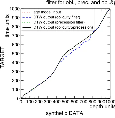
2.5 Testing the DTW algorithm with synthetic data . . . 55

2.5.1 Experiment #1: Testing variable sedimentation rates . . . 58

CONTENTS viii

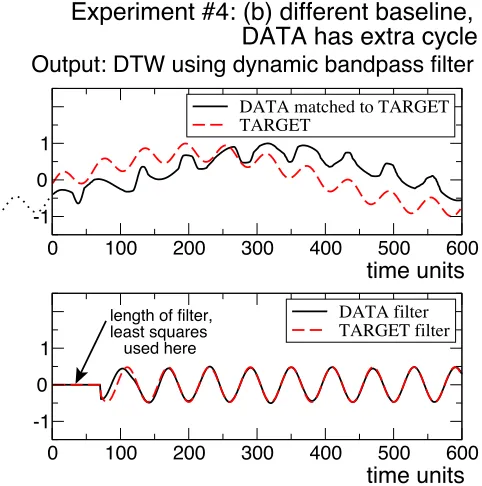
2.5.3 Experiment #4: Testing bandpass filtering as correlation tool . . . 62

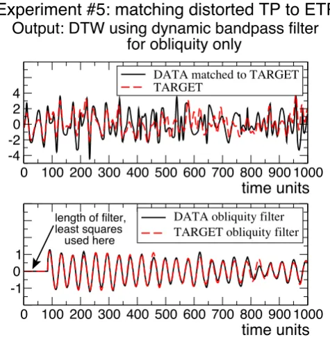
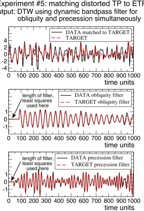
2.5.4 Experiment #5: bandpass filtering of multiple frequencies . . . . 64

2.6 Using the DTW algorithm with geological data: a case study . . . 68

2.6.1 Methods and parameters used for DTW age model generation . . 70

2.6.2 Comparison of initial and generated age models . . . 71

2.7 An automated tuning approach: Conclusions . . . 83

Chapter 3 Extending the astronomical calibration into the Eocene 86 3.1 Introduction . . . 86

3.2 A new time scale for the Middle and Late Eocene . . . 88

3.2.1 Background and introduction to ODP Site 1052 . . . 88

3.2.2 Magnetostratigraphy . . . 90

3.3 XRF scanning . . . 90

3.3.1 Methods and Parameters . . . 91

3.3.2 Results from XRF scanning . . . 93

3.4 A new rmcd scale . . . 95

3.4.1 Differences in relative stratigraphic thickness between holes . . . 95

3.4.2 XRF and proxy results for the rmcd composite . . . 97

3.5 Volcanic Ash Layers . . . 98

3.6 Cyclicity in the depth-domain . . . 102

3.7 Astronomical Tuning . . . 103

3.7.1 Strategy . . . 103

3.7.2 Time scale development . . . 106

3.8 Sedimentation rates and a possible hiatus . . . 108

3.9 Spectral Analysis . . . 109

3.9.1 Amplitude modulation patterns obtained by complex demodula-tion . . . 110

3.10 Implications for magnetostratigraphy . . . 114

3.11 Results from XRF analysis of Site 1052: Summary . . . 115

3.12 Comparison with data from ODP Leg 177, Site 1090B . . . 116

3.13 Summary of analysis of data from Site 1090 . . . 126

CONTENTS ix

Chapter 4 Stable isotope data from ODP Leg 171B, Site 1052 128

4.1 Introduction . . . 128

4.2 Methods used for generation of stable isotope record . . . 129

4.3 Benthic stable isotopes fromNuttalides truempyi . . . 131

4.3.1 Comparison ofNuttalides truempyiand planktonic data . . . 133

4.3.2 Temperature estimates from benthic and planktonic oxygen iso-topes and carbon isotope gradients . . . 135

4.4 Extending the benthic isotope record . . . 139

4.5 Obliquity variations in the benthic oxygen isotope record . . . 142

4.6 Isotope data from bulk fine fraction . . . 144

4.7 Unusual stable isotope and lithological events at Site 1052 . . . 145

4.8 Conclusions based on stable isotope data . . . 148

Chapter 5 Extracting astronomical parameters from geological data 149 5.1 Introduction . . . 149

5.2 Extracting tidal dissipation and dynamical ellipticity from geological data 151 5.2.1 What causes tidal dissipation? . . . 152

5.2.2 Current estimates for tidal dissipation . . . 153

5.2.3 Astronomical frequencies and parameters . . . 154

5.2.4 Method to detect changes inp: interference patterns and beats . 157 5.2.5 Correcting for astronomical tuning to a target . . . 160

5.2.6 Semi-analytical approximation of Laskar’s solution . . . 162

5.2.7 Principles of tuning correction . . . 165

5.2.8 Analytical precision . . . 166

5.2.9 Processing of data . . . 166

5.2.10 Sensitivity of the interference method . . . 168

5.2.11 Modelling with geological data . . . 168

5.2.12 Analysis from 0-5 Ma . . . 173

5.2.13 Increasing the time interval of analysis . . . 173

5.2.14 Discussion . . . 176

5.3 Evaluating different astronomical calculations using geological data . . . 180

5.3.1 Why is there a need for an improved astronomical solution? . . . 180

5.3.2 Comparison of astronomical solutions: La2001 and La1993 . . . . 181

CONTENTS x

5.3.4 Differences in obliquity amplitude modulation . . . 193

5.3.5 Differences in the eccentricity modulation . . . 196

5.3.6 Analysis of geological data and their limitations . . . 196

5.3.7 Feature comparison of data and models from 18 to 28 Ma . . . 198

5.3.8 Obliquity amplitude modulation . . . 199

5.3.9 Eccentricity and climatic precession amplitude modulation . . . 201

5.3.10 Comparison of data and models from 33 to 38 Ma . . . 203

5.3.11 Comparison of solution La2001 with an independent calculation 204 5.3.12 Is a rare orbital anomaly the trigger for the unusual oxygen and carbon isotope (“Mi-1”) event? . . . 207

5.3.13 Findings from evaluation of astronomical solutions . . . 207

5.4 Conclusions . . . 209

Chapter 6 Conclusions and future work 210 6.1 Introductory remarks . . . 210

6.2 Conclusions: An automated astronomical tuning method . . . 210

6.3 Conclusions: A new age calibration of the late Eocene . . . 211

6.4 Conclusions: A detailed stable isotope record from the Eocene . . . 212

6.5 Conclusions: Extraction of orbital parameters encoded in geological data 212 6.6 Future work . . . 213

References 216

Appendices 230

Appendix A Raw XRF data from ODP 171B-1052 230

List of Figures

1.1 Orbital elements of the Earth’s movement around the sun. . . 12

1.2 Eccentricity curve and frequency analysis . . . 16

1.3 Obliquity curve and frequency analysis . . . 19

1.4 Climatic precession curve and frequency analysis . . . 20

1.5 Joint time-frequency analysis of astronomical model 0-10 Ma . . . 24

1.6 Estimated changes in the obliquity and climatic precession periods . . . 26

2.1 Comparison of independent astronomical tuning with geomagnetic time scale . . . 34

2.2 Comparison of three different astronomical solutions to demonstrate obliquity and climatic precession interference . . . 36

2.3 Illustration of different types of orbital targets curve . . . 38

2.4 Depth to time conversion with constraints on sedimentation rate and continuity . . . 40

2.5 Comparing pattern matching based on correlation coefficients and fit-ting peaks . . . 43

2.6 An example of using bandpass filtering for correlation . . . 45

2.7 Typical local continuity constraints for dynamic time warping . . . 52

2.8 Generalised constraints for DTW tuning . . . 56

2.9 Synthetic input data for DTW algorithm, experiment #1 . . . 58

2.10 DTW algorithm output for experiment #1 . . . 60

2.11 Synthetic input data for DTW algorithm, experiment #2 . . . 61

2.12 DTW algorithm output for experiment #2 . . . 61

2.13 Synthetic input data for DTW algorithm, experiment #3 . . . 61

2.14 DTW algorithm output for experiment #3 . . . 62

LIST OF FIGURES xii

2.16 DTW algorithm output for experiment #4 (a) . . . 63

2.17 DTW algorithm output for experiment #4 (b) . . . 64

2.18 Synthetic input data for DTW algorithm, experiment #5 . . . 65

2.19 DTW algorithm output for experiment #5 . . . 66

2.20 DTW algorithm output for experiment #5 . . . 67

2.21 DTW algorithm age models for experiment #5 . . . 68

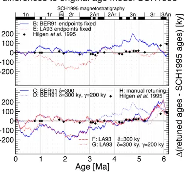
2.22 Tuning results for ODP 138-846 GRAPE density: age differences with orig-inal tuning . . . 73

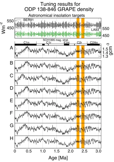
2.23 Tuning results for ODP 138-846 GRAPE density 0-3.1 Ma . . . 75

2.24 Tuning results for ODP 138-846 GRAPE density 3.1-6.2 Ma . . . 76

2.25 Tuning results for ODP 138-846 GRAPE density: obliquity filters . . . 77

2.26 Tuning results for ODP 138-846 GRAPE density: precession filters . . . . 78

2.27 Tuning results for ODP 138-846 GRAPE density: sedimentation rates . . . 79

2.28 Tuning results for ODP 138-846 GRAPE density: Blackman-Tukey spec-tral estimates . . . 80

2.29 Tuning results for ODP 138-846 GRAPE density: MTM evolutive spectra . 82 2.30 Comparison of benthic oxygen isotope data from ODP Legs 138 and 154 83 3.1 Location Map for ODP 171B drilling sites . . . 89

3.2 Photograph of the container laboratory housing the XRF Core Scanner . 92 3.3 Comparison of chemical CaCO3 measurements and XRF measurements of Ca, Fe, and Ca/Fe . . . 94

3.4 Relative amount of stretching and squeezing performed to create the rmcd scale . . . 96

3.5 Stacked XRF data . . . 99

3.6 Evolutive spectral analysis in the depth domain for colour reflectance . . 103

3.7 Evolutive spectral analysis in the depth domain for Ca/Fe XRF data . . . 104

3.8 Astronomically tuned XRF, MS, and lightness data . . . 107

3.9 Cross-spectral analysis between astronomically tuned XRF Ca /Fe data and the astronomical target curve. . . 110

3.10 Complex demodulations for XRF data and astronomical models . . . 112

3.11 Cross-spectral analysis obtained for the amplitude modulation at the cli-matic precession frequency. . . 113

LIST OF FIGURES xiii

3.13 Location Map for ODP 177 Site 1090 . . . 118

3.14 Bio- and magnetostratigraphic age model for Site 1090, Hole B . . . 119

3.15 Core photograph from ODP 177, Site 1090, Hole B . . . 122

3.16 Comparison of data from Sites 1052 and 1090 . . . 124

3.17 Cross-spectral analysis between astronomically tuned XRF Ca/Fe data and light reflectance data . . . 126

4.1 Stable isotope record from benthic speciesNuttalides truempyi . . . 132

4.2 Comparison of benthic and planktonic stable isotope records from foraminifera . . . 134

4.3 Temperature estimates from benthic and planktonic foraminifera . . . . 137

4.4 Difference between planktonic and benthicδ13C . . . 138

4.5 Extended stable isotope record. . . 140

4.6 Comparison of benthic oxygen isotope ratios and XRF Ca /Fe ratios . . . 143

4.7 Benthic isotope values and bulk fine fraction measurements . . . 145

4.8 Isotope excursion event identified in C17n.1n . . . 146

5.1 Interference pattern from two astronomical solutions . . . 159

5.2 Illustration of tuning effect on frequencies . . . 161

5.3 Sensitivity of interference method . . . 169

5.4 Interference pattern results from tuning to La93(1,1)and comparing with La93(1,0) . . . 171

5.5 Interference pattern results from tuning to La93(1,1)and comparing with La93(1,−2) . . . 172

5.6 Best fitting interference model 0-5 Ma . . . 174

5.7 Best fitting solution for 0-11.5 Ma and 17.5-24 Ma . . . 175

5.8 Comparison of obliquity calculations La1993 and La2001 from 0-20 Ma . 187 5.9 Comparison of eccentricity calculations La1993 and La2001 from 0-20 Ma 188 5.10 Joint time-frequency wavelet analysis for La2001 from 0-50 Ma . . . 190

5.11 Joint time-frequency wavelet analysis for La1993 from 0-50 Ma . . . 191

5.12 Difference plot of joint time-frequency wavelet analyses for La2001 and La1993 from 0-50 Ma . . . 192

LIST OF FIGURES xiv

5.14 Comparison of ∼100ky eccentricity amplitude complex demodulation from La1993 and La2001 for 0-50 Ma . . . 195 5.15 Location Map of ODP sites used for comparison of geological data and

astronomical solutions . . . 197 5.16 Comparison of obliquity amplitude modulation between astronomical

models and data from ODP 154 (18-30 Ma) . . . 200 5.17 Comparison of amplitude modulation of 400ky eccentricity cycle

be-tween astronomical models and data from ODP 154 (18-30 Ma) . . . 202 5.18 Obliquity amplitude modulation comparison for astronomical models

and data from ODP 171 and 177 (33-40 Ma) . . . 205 5.19 Comparison of eccentricity calculations La2001 and Varadiet al.

(calcu-lation R10) from 0-50 Ma . . . 206 5.20 Comparison of orbital calculations and the age of the Mi-1 stable isotope

event . . . 208

List of Tables

1.1 Fundamental orbital frequencies . . . 14

1.2 Principal eccentricity frequency components . . . 16

1.3 Principal obliquity frequency components . . . 18

1.4 Principal climatic precession frequency components . . . 19

1.5 Orbital amplitude modulation terms . . . 23

3.1 Magnetic reversals from Site 1052 and their depth uncertainty on the rmcd (revised metres composite depth) scale. . . 91

3.2 Identified ash layers and their position in each hole . . . 101

3.3 Comparison of relative age estimates of magnetic reversals from Sites 1090 (Hole B) and 1052 . . . 125

5.1 Principal frequencies in the astronomical solution La93(1,0) . . . 155

5.2 Summary of constants . . . 162

5.3 Interference results 0-5 Ma . . . 176

5.4 Interference results 0–6.5 Ma . . . 177

5.5 Interference results 0–8 Ma . . . 177

5.6 Interference results 0–9 Ma . . . 177

5.7 Interference results 0-11.5 Ma . . . 178

5.8 Interference results 0–11.5 Ma and 17.5i–24 Ma . . . 178

5.9 Leading eccentricity terms for La1993 and La2001 . . . 183

5.10 Leading obliquity terms for La1993 and La2001 . . . 184

5.11 Precession frequencies for La1993 and La2001 . . . 185

A.1 XRF measurements from Leg 171B, Site 1052, Hole A . . . 231

A.2 XRF measurements from Leg 171B, Site 1052, Hole B . . . 232

LIST OF TABLES xvi

A.4 XRF measurements from Leg 171B, Site 1052, Hole F . . . 234

B.1 Mapping pairs from mbsf to rmcd for Site 1052, Hole A . . . 236

B.2 Mapping pairs from mbsf to rmcd for Site 1052, Hole B . . . 237

B.3 Mapping pairs from mbsf to rmcd for Site 1052, Holes C and D . . . 238

B.4 Mapping pairs from mbsf to rmcd for Site 1052, Hole F . . . 239

B.5 Mapping pairs from rmcd to age for Site 1052 . . . 240

C.1 Interpolated and stacked XRF and colour measurements from Leg 171B, Site 1052 . . . 242

D.1 Benthic foraminiferal stable isotope measurements, Site 1052, Hole A . . 244

D.2 Benthic foraminiferal stable isotope measurements, Site 1052, Hole B . . 245

D.3 Benthic foraminiferal stable isotope measurements, Site 1052, Hole F . . 246

D.4 Stable isotope bulk sediment measurements, Site 1052, Hole B . . . 247

D.5 Stable isotope bulk sediment measurements, Site 1052, Hole F . . . 248

E.1 Interpolated colour reflectance data from Leg 177, Site 1090, Hole B . . . 250

Chapter 1

Introduction, historical overview

and astronomical theory

1.1 Introduction

1.2 Outline of Dissertation 2

1.2 Outline of Dissertation

1.2.1 Chapter one outline

The remainder of chapter one provides a historical overview of the developments that led to the modern understanding of geological time. Chapter one then outlines the historical developments that were specifically concerned with the use of astronomical variations that are recorded in the geological record. A brief summary is given of recent developments in the use of “cyclostratigraphy”. An important part of this chapter is a summary of astronomical theory as far as it relates to orbital patterns that can be observed in the geological record. A short summary is given of how long, continuous high-resolution geological records are generated from deep-marine sediments.

1.2.2 Chapter two outline

Chapter two provides a theoretical framework describing how it is possible to quanti-tatively correlate geological data with templates given by astronomical calculations. A speech-recognition algorithm is adapted to compute age-depth relationships accord-ing to certain criteria and constraints. This method is first tested with synthetic data, and then applied to real geological data. The advantages and limitations of an auto-mated approach to stratigraphic and time scale correlation are demonstrated.

1.2.3 Chapter three outline

1.2 Outline of Dissertation 3

1.2.4 Chapter four outline

Chapter four presents additional stable oxygen and carbon isotope data that were gen-erated from the same material as that discussed in chapter three. These data support the conclusions reached in chapter three, and provide an independent check of the plausibility of the age model developed therein. These data provide a high-resolution record of climatic variations over intervals of the late Middle and Late Eocene for the first time.

1.2.5 Chapter five outline

Chapter five deals with the extraction of astronomical parameters from geological data over the last∼37 million years. It thus presents a complementary approach to work pre-sented in chapters three and four, where astronomical calculations were used to gen-erate a geological time scale. Astronomically calibrated geological data are analysed to extract parameters that are required for the calculation of detailed astronomical mod-els. Very small changes in the Earth’s precession constant are extracted by developing a new interference method. This technique leads to the extraction of the long-term evo-lution of the tidal dissipation and dynamical ellipticity parameters of the Earth for the last 25 million years.

Geological data spanning the last∼37 million years are used to extract long term amplitude modulation patterns of the climatic signal. A comparison of the long term amplitude modulation derived from published astronomical calculations, and those derived from a new calculation (J. Laskar, 2001, unpublished), shows that the geological record supports the validity of the new solution. This study forms the basis for a further extension of the astronomical calibration of the geological time scale into earlier parts of the Paleogene.

1.2.6 Chapter six outline

1.3 The age of the Earth - A historical overview 4

1.3 The age of the Earth - A historical overview

Since this dissertation is concerned with the determination of the duration and age of sedimentary layers, it is appropriate to give a short historical overview of the develop-ments that led to the modern understanding of geological age and stratigraphy. Due to its significance for observations of natural processes, and its direct impact on religious and philosophical thinking, the age of the Earth and its sedimentary layers has been the subject of many historical accounts and hypotheses.

The earliest known records that report geological observations, relating to the time and duration of landscape forming processes, date back as far as the sixth century B.C. The Greek philosopher Xenophanes of Colophon observed shells embedded into the cliffs on the island of Malta, and proposed that the land was periodically covered by the sea [1]. He recognised the significance of fossils as a record of former life, and in-terpreted the layers of sedimentary rocks as the result of sediment accumulating on the bottom of the sea over a long interval of time. Around 450 B.C. the Greek histo-rian Herodotus travelled through the Nile river valley and described and named the Nile delta [2]. His observation of sedimentary layers, and embedded fossils, led him to conclude that the Nile delta must have originated from a large number of floods, representing at least several thousands of years.

During the Renaissance, Leonardo da Vinci (1452-1519) described sea shells from the Apennine Mountains, and postulated that these were the remains of organisms that had been buried by river muds from the Alps, before they were petrified and later uplifted [3]. Following the rise of the power of the western Church, the knowledge ac-cumulated from previous observations was suppressed and ignored during medieval times, when several theologists used a literal interpretation of the book of Genesis to “calculate” the age of the Earth. The most cited example is probably that of Archbishop of Armagh James Ussher, who claimed in 1650 that the year of creation was 4004 B.C. [4]1_.

It was not until the pioneering works of the famous Scottish geologist James Hut-ton (1726-1797) [5; 6] that it was recognised again that the sedimentary deposits on the surface of the Earth resulted from continuing geological processes, rather than be-ing caused by sbe-ingle “catastrophic” events. Hutton observed how weatherbe-ing, erosion

1_{As a historical curiosity, it was Ussher’s contemporary Dr. John Lightfoot (1602-1675), Vice Chancellor}

1.3 The age of the Earth - A historical overview 5

and sedimentation slowly form soft sediments, which are subsequently slowly buried, heated, compressed, and uplifted to complete the sedimentary cycle. He appreciated that the Earth must be immensely old, and famously stated that

“The result, therefore, of our present enquiry is that we find no vestige of a beginning, no prospect of an end.”

Together with the subsequent support of Hutton’s theories by Charles Lyell (1797-1875) through his influential publication of “Principles of Geology” [7], it was the work of the engineer and surveyor William Smith (1769-1839), through his analysis and map of faunal successions in England and Wales [8], that laid the foundation for modern stratigraphic approaches in the geological sciences. His work, in turn, forms the basis for approaches to the subdivision of geological strata according to relative time. By then it was firmly established within the geological community that sedimentary rocks rep-resent an unfathomably long amount of time. The first calculations of the total age of the Earth were made, accounting for the thickness of sediment observed at the Earth’s surface, and assuming that the present rate of erosion and deposition was representa-tive of the past. This uniformitarian approach led to estimates of the age of the Earth of the order of millions to hundreds of millions of years.

In 1862, William Thomson (1824-1907), later Lord Kelvin, made public a calcula-tion of the age of the Earth based on a thermodynamic cooling model [9]. His original age limit was 20 to 400 million years. Considering the physical principles known at the time, and calculating the dissipation of energy from the Sun, he later arrived at an age estimate of the Earth of between 24 and 40 million years. This age was considered much too young by contemporary geologists, including Charles Darwin, but had an enormous impact due to Lord Kelvin’s authority in many fields of science.

1.4 A history of cyclostratigraphy and “Milankovitch” theory 6

The basis for a modern biostratigraphic approach was formalised by William Smith, but it was the discovery of sea-floor spreading (see, e.g., Hess, 1962 [13]), and the mag-netic reversal record (Vine and Matthews, 1963 [14]), that provided an important pre-requisite for the modern stratigraphic approach in the Earth sciences, where radiomet-ric decay methods allow the dating of bio- and magnetostratigraphic events that can potentially be correlated globally (Coxet al.(1963) [15]). The next section outlines the history of the development of a cyclostratigraphic approach, where the relative dura-tion of cyclical patterns in geological records is estimated and correlated by using as-tronomical theory.

1.4 A history of cyclostratigraphy and “Milankovitch” theory

It is appropriate to give a separate historical overview of the scientific thoughts and discoveries that led to the development of the astronomical theory of palaeoclimates and cyclostratigraphy, i.e. the use of astronomical cycles, recorded in geological suc-cessions, as a measure of time. The recognition of changes in climate, reflected in sed-imentary rocks, has been the subject of scientific interest for at least the last 170 years, and predates the “modern” approaches of Lord Kelvin, the discovery of radioactivity, and the invention of radiometric dating. Astronomical theory was first invoked by sci-entists who wanted to explain the occurrence of glaciations in the past, rather than to examine the question of geological time. A thorough historical overview of the quest to solve the mystery of the ice ages was given by Imbrie and Imbrie (1979) [16]. Their book covers the discoveries up to the late 1970s, and here only a brief summary is given for the early history.

1.4 A history of cyclostratigraphy and “Milankovitch” theory 7

causes of ice ages in the 1860s.

Croll was arguably one of the most important figures in the historical development of the relationship between astronomical theory and climate. Building on astronom-ical calculations by Le Verrier (1856) [20], he published the influential “Climate and time in their geological relations” in 1875 [21]. The contribution of Croll was of great significance because, for the first time, he considered the combined effects of the axial tilt and the precession of the equinoxes of the Earth’s orbit, in addition to the orbital eccentricity, on the seasonal variations in insolation during perihelion and aphelion (those points on the orbit of the Earth closest to, and furthest from, the Sun, respec-tively). Croll developed detailed models of how the volume of ice varies in time, and proposed that the initiation of glacial stages is controlled by cold northern hemisphere winters, and short, hot summers. He was the first to consider the effects of albedo as a positive feedback mechanism. His book contains many ideas about ocean circula-tion and climatology that are still valid. It would be fair to say that Croll was one of the founders of quantitative palaeoceanography.

Subsequently, however, some of Croll’s predictions and ideas dissatisfied geologists and meteorologists alike, and led to the temporary abandonment of his ideas. One of Croll’s theories was that the last glacial interval ended 80 thousand years ago, in conflict with new evidence at the time that this time estimate should be much younger. Meteo-rologists noted that Croll’s proposed changes in the heating from the Sun, according to astronomical variations, would cause a change in climate of much smaller amplitude than required, and opposed the implication from Croll’s theory that ice ages occurred at alternating times in the southern and northern hemisphere. Interestingly, though, his ideas still led to a revival of the idea that rhythmic sedimentary alternations could be interpreted as a measure of time. This interpretation was proposed by Gilbert in 1895 [22], who attributed cyclic Cretaceous strata to a precessional forcing.

Although several studies challenged Croll’s theory that long, cold winters, and short, hot summers favour glaciations, and in fact arrived at the opposite conclusion [23; 24], it was not until the work of Milankovitch during the 1920s through the 1940s that a detailed mathematical approach to the change of insolation became available.

The Serbian mathematician and geophysicist Milutin Milankovitch2 (1879-1958) advanced the theory of the ice ages by computing the solar irradiance at different

1.4 A history of cyclostratigraphy and “Milankovitch” theory 8

itudes and different seasons of the year [25; 26]. As a result, he proposed what is now known as the “Milankovitch” theory of glaciations, where the variation in solar radi-ation at high northern latitudes is responsible for the waxing and waning of ice. In particular, Milankovitch proposed that conditions favouring glaciations are short cold summers, thus preventing the melting of ice accumulated over the winter, aided by en-hanced evaporation and precipitation during mild winters. According to Milankovitch, to achieve short and cold summers, the necessary conditions include a northern hemi-sphere summer during aphelion, a minimum in obliquity leading to a weaker seasonal contrast, and a maximum in eccentricity, leading to an increased distance between the Earth and the Sun at the aphelion during summer.

Milankovitch’s theory was not well received at the time, partly for the same reasons that Croll’s ideas were criticised. Without consideration of the uneven distribution of land masses between the northern and southern hemispheres, and without consid-ering the complex interplay of ocean circulation patterns and climate, Milankovitch’s theory would predict alternating southern and northern hemisphere glaciations. Later research showed that the Quaternary ice age cycles occurred approximately every 100 thousand years (ky)3_{, which was at odds with Milankovitch’s predictions for the}

strongest frequency components, which are in fact the obliquity and precession fre-quency components, rather than the much weaker∼100 ky eccentricity component.

The essence of Milankovitch’s astronomical theory, i.e. that variations in insolation drive changes in climate, was finally accepted following the analysis of deep-sea sed-iment cores in the 1970s, which showed the presence of the obliquity and precession components in addition to the eccentricity component. Following the pioneering sta-tistical evaluation of cyclic patterns in the rock record by Schwarzacher [27; 28], Hayset al.(1976) [29] published a seminal paper that demonstrated statistically the presence of obliquity and precession cycles in the geological record. Their analysis was made pos-sible by advances in the analysis of stable isotope ratios by Urey and later by Emiliani (1955, 1966) [30; 31]. The paper by Hayset al.spawned a large number of studies in-vestigating the relationship between astronomy, climate and time that have continued until the present, although there are still contrasting views on the exact nature of astro-nomical forcing and time lags between the forcing and the recording in the geological record (see, e.g., Henderson and Slowey (2000) [32] and Herbertet al.(2001) [33]).

3_{Throughout this thesis, durations are denoted by ky for thousands of years, My for millions of years}

1.5 The development of detailed astronomically calibrated time scales 9

Following the work done in the early 1970s, the history of the “ice ages” was more thoroughly investigated and resulted in many ground-breaking publications, includ-ing the CLIMAP and SPECMAP projects [34–37]. The discovery of split peaks in the precession frequency band in geological data also tied in neatly with more accurate calculations of the Earth’s orbit by Berger (1978) [38], which further enhanced scientific interest in the subject.

1.5 The development of detailed astronomically calibrated

time scales

After the presence of orbitally related variations in the climatic record of the Quaternary was confirmed, the search for astronomical frequencies was extended to older parts of the geological record. It can be argued that advances in the use of astronomical cy-cles as a measure of time were slowed by the initial close linkage between astronomical variations, and records and causes of the ice ages. As shown by Pisias and Moore (1981) [39], and investigated later by Ruddimanet al.(1986) [40], the Quaternary shows an un-usually strong∼100 ky long “sea-saw” pattern in marine climate proxies. This regime was preceded (before∼1.3 Ma) by a more dominant obliquity and climatic precession component with periodicities of∼41 ky, and 23 ky and 19 ky, which can be more easily reconciled with the relative amplitude of these cycles in the insolation forcing.

This discovery was important, because to some extent it allowed the separation of the detailed investigation of the causes of the ice ages and climatic variations on the one hand, and the use of orbitally controlled cyclicity in the geological record as a tool to estimate time on the other hand. This process was initiated by the landmark paper of Shackleton et al.(1990) [41], which proposed for the first time an absolute dating of the Brunhes-Matuyama magnetic reversal that was based on an astronomical cali-bration, and which implied an age of 780 ka, approximately 5-7% older than previous radiometric estimates. This older age was later confirmed by high-precision40_Ar/39_Ar

dating of lavas close to the Brunhes-Matuyama boundary [42] and demonstrates the use of astronomically calibrated time scales.

1.6 Astronomical theory 10

of the astronomically calibrated Neogene geological time scale (Hilgen, 1991 [43; 44]). These studies were significant because, for the first time, they allowed the integration of astronomically calibrated ages with the geomagnetic polarity time scale (GPTS) by Cande and Kent (1992,1995) [45; 46] (also reviewed by Kent, 1999 [47]). This is only one example of how the detailed high-resolution study of cyclic variations in the sedimen-tary record can have an impact on other fields in the Earth sciences.

During the course of the last fifteen years, a very large number of studies have found evidence of orbitally controlled cyclicity in the geological record at intervals through-out the Phanerozoic. Some representative (but non-exhaustive) examples can be given from the Cenozoic era [41; 43; 44; 48–55], the Mesozoic era [56–63], as well as the Pale-ozoic [64]. There have now also been a large number of attempts to contribute to the understanding of the response of the climate system to orbital forcing through mod-elling studies (see, e.g., Shortet al.(1991) [65]). Detailed insights into the behaviour of the climate system in the past have also been obtained from ice cores (see, e.g., Barnola

et al. (1987) [66] and Petit et al. (1999) [67]). Records of past atmospheric composi-tion, obtained from air bubbles trapped inside the ice, provide a very important direct archive of climate change over the last few hundred thousand years, and have recently been used to gain an important understanding of the complex interplay between or-bital forcing, ice dynamics, and the climate system (Shackleton, 2000 [68]). It is beyond the scope of this overview to give a detailed account of all publications, but due to the recognition of the significance and prevalence of orbitally controlled cycles in the ge-ological record, there now exist several collections of papers that can be consulted to obtain references to a significant part of the relevant literature [69–74].

1.6 Astronomical theory

1.6 Astronomical theory 11

al.(1978,1991,1992,1993) [38; 80–82], Loutre (1993) [78], Laskar (1986,1988,1990,1993) [83–86], and deSurgy and Laskar (1997) [87].

1.6.1 Celestial mechanics

The time-varying motion of the planets and other satellites around the Sun is controlled by their mutual gravitational interaction. It can be described by Newton’s laws, cor-rected by Einstein’s principles of general relativity. The behaviour of the solar system is complex, because it is posed as an n-body problem (which can only be solved numer-ically), and is further complicated by physical parameters such as the tidal dissipation of energy as well as the detailed distribution of mass within each body. As a result of this complexity, the planets do not follow stationary orbits around the Sun, but undergo quasi-periodic as well as chaotic motions that, from a climatic point of view, affect the amount, distribution, and timing of solar radiation received at the top of the Earth’s atmosphere.

At any given time, the orbit of a body can be described by six parameters, which are traditionally the six “Keplerian orbital elements”. These parameters define the po-sition, shape, and orientation of the orbit, and the location of a body on this orbit, with respect to a frame of reference. The trajectory of the orbiting body follows an ellipse which, in the case of the solar system, has the Sun located at one focal point. Due to the gravitational interaction of the different planets, the orientation and dimension of this ellipse change over time.

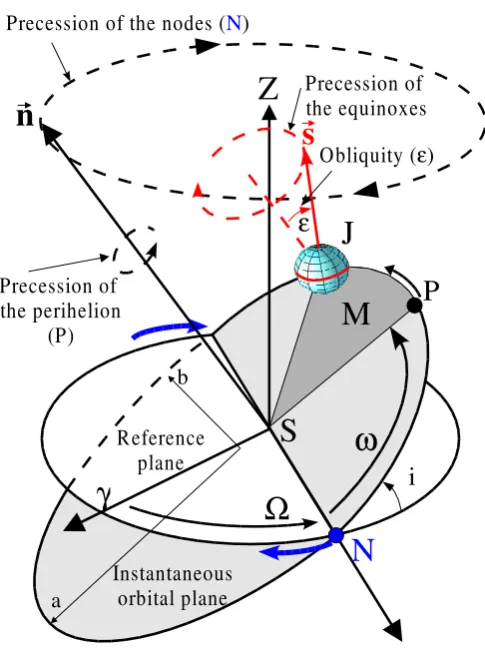
Figure 1.1 illustrates the definition of the six Keplerian elements, as applied to the Earth on its orbit. The reference plane, which is fixed with respect to the stars, is typ-ically chosen as the orbital plane of the Earth at a particular time (e.g. 1850, 1950 or 2000 A.D.), and is called the “ecliptic of epoch”. Alternatively, for certain calculations, it can be chosen to coincide with the invariable plane of the solar system, which is the “average” plane defined by the total angular momentum of the solar system. This “in-variant” plane almost coincides with the orbital plane of Jupiter due to its large mass. The reference plane is defined by two axes. One of these is typically the position of the mean vernal (spring) equinox on the reference plane at a given time, denoted byγ, while the second axis is perpendicular to this axis as well as to the reference plane (“Z”), both originating from the position of the Sun (“S”) on the reference plane.

1.7 The origin of orbital frequencies 12

i

M

P

Ω

N

ω

γ

Z

J

S

s

n

ε

a

b Reference

plane

Instantaneous orbital plane Precession of the nodes (N)

Precession of the equinoxes

Precession of the perihelion

(P)

Obliquity (ε)

Figure 1.1: Orbital elements of the Earth’s movement around the sun.

axis of the orbital ellipse, which corresponds to the average radius. The eccentricitye of the ellipse is defined as e = √a2_a−b2, whereb is the semi-minor axis of the ellipse. The inclination of the orbit with respect to the reference plane is given by the anglei. The position of the ascending node N is specified by the angle Ω(“longitude of the node”), measured from the fixed direction in the reference plane (γ). The parameter !

ω specifies the position of the moving perihelionP (the closest approach to the Sun) and is defined asω! =Ω+ω(“longitude of the perihelion”). Finally, the sixth Keplerian elementλspecifies the position of the orbiting body (“J”) on its elliptical orbit, and is defined asλ=ω_!+M, whereM(“mean anomaly”) is an angle which is proportional to the areaSP J(Kepler’s third law).

1.7 The origin of orbital frequencies

1.7 The origin of orbital frequencies 13

fixed for all times. In this situation, the only Keplerian element that would change over time would beλ, which describes the position of the body on its orbit. In this case, the position and velocity of the orbiting body would vary according to the Keplerian laws of motion around a fixed ellipse.

However, gravitational interactions between all bodies of the solar system cause changes in the shape and orientation of the elliptical orbit on various time scales, which are typically of the order of104₋₁₀6 _{years. From a climatic point of view, the relevant}

variations are those obtained after averaging the planetary orbits over their long-term orbital periods. These are called secular variations, and can be described by a set of fundamental frequencies.

The variation in the orbital elements that characterises the secular variations can be separated into two types, which are related to different types of precession movements. The first group is the variation within the orbital plane, and is described by the varia-tion of the eccentricitye, and the rotation of the location of the perihelion, described byω. The second group is the variation of the orientation of the orbital plane, and is de-scribed by the inclination anglei, and the location of the ascending nodeN, described by Ω. These oscillations are coupled such that one can investigate the behaviour of these parameters as pairs(e,ω)and(i,Ω).

1.7.1 Fundamental frequencies of the solar system

By computing the orbital elements for the main eight planets (Pluto is excluded), one obtains eight characteristic modal frequencies for each of the paired elements (e,ω) and(i,Ω). Table 1.1 lists these fundamental frequencies, as estimated by Laskar (1990) [85] over the last 20 My. Individual frequenciesgi are related to variations in the pair

(e,ω), while frequenciessiare related to variations in the pair(i,Ω). The individualgi andsifrequencies arise as eigenvalues if Poisson equations are used to expand the or-bital elements for the eight planets. As eigenvalues of a matrix, they are not strictly asso-ciated with a particular planet. However, since the matrix from which they are obtained has a diagonal structure, suppressing a planet removes one set of frequencies while not changing the other frequencies significantly (Laskar, personal communication). Thus, the indices in gi, si can be used to indicate which planet provides the strongest con-tribution to a particular frequency (g1, s1 correspond to Mercury,g3, s3 to Earth, and

1.7 The origin of orbital frequencies 14

Fundamental orbital frequencies related to(e,ω) related to(i,Ω)

term frequency Period term frequency Period associated

(##_{/a) (ky) (}##_{/a) (ky) Planet}

g1 5.596 231.0 s1 -5.618 230.0 Mercury

g2 7.456 174.0 s2 -7.080 183.0 Venus

g3 17.365 74.6 s3 -18.851 68.7 Earth

g4 17.916 72.3 s4 -17.748 73.0 Mars

g5 4.249 305.0 s5 0.000 Jupiter

g6 28.221 45.9 s6 -26.330 49.2 Saturn

g7 3.089 419.0 s7 -3.005 431.0 Uranus

g8 0.667 1940.0 s8 -0.692 1870.0 Neptune

Table 1.1: Fundamental orbital frequencies of the precession motions in the solar sys-tem, computed as mean values over 20 million years by Laskar (1990) [85]. Thegi and si are eigenvalues that characterise the evolution of the orbital elements(e,ω) and (i,Ω), respectively, and are loosely associated with the eight planets considered, i.e.g1, s1 correspond to Mercury, andg8, s8

corre-spond to Neptune. Periods in years can be calculated from arcseconds per year asperiod(a) = _{f requency}360×60×₍60_!!/a).

counter-clockwise if viewed from the “north” of the orbital axis (shown in figure 1.1). In contrast, seven out of the eightsiterms are negative, indicating that the position of the nodes, which mark the intersection of the orbital plane with the reference plane, regress (rotate clockwise). The frequencys5is zero because the invariant plane is close

to the orbital plane of Jupiter due to Jupiter’s large mass.

1.7.2 General precession of the Earth

1.7 The origin of orbital frequencies 15

only the precession component has a significant effect.

With respect to the fixed stars, the frequency of this precessional cycle is denoted asp, and has a period of approximately 25.8 ky. The precession of the Earth’s spin axis has several effects on the Earth’s climate system, one of which is that the position of the seasons with respect to the Earth’s orbit, defined by the solstices and equinoxes with respect to the perihelion and aphelion of the orbit, changes over time. For this reason the precession of the Earth’s spin axis is also called the “precession of the equinoxes”. This precession will be discussed in more detail in one of the following sections.

As shown in figure 1.1, the precession of the Earth’s spin axis traces out a cone that forms an angle with the Earth’s orbital plane. This angle is the obliquity (tilt) of the Earth, and is denoted by%. This angle changes due to the combined effect of the pre-cession of the Earth’s spin axis and the changing orientation of the Earth’s orbital plane, which will be discussed in more detail in a following section.

As a first order approximation, the fundamental frequenciesgiandsi can be used together with the precession constantpto explain the origin of almost all periodicities that affect the climate system. They arise from “beats” between the fundamental fre-quencies. In detail, though, additional resonance terms are present in the solar system, which lead to the presence of chaos (Laskar, 1990 [85]). The presence of chaos in the solar system has important consequences, which will be discussed separately in sec-tion 1.7.9. The following secsec-tions discuss how the three orbital parameters eccentricity, obliquity, and climatic precession, which are involved in the calculation of the solar radiation, are related to the fundamental frequencies of the solar system

1.7.3 Eccentricity

1.7 The origin of orbital frequencies 16

Five leading terms for Earth’s eccentricity term frequency Period Amplitude

(##_{/a) (ky)}

g2−g5 3.1996 406.182 0.0109

g4−g5 13.6665 94.830 0.0092

g4−g2 10.4615 123.882 0.0071

g3−g5 13.1430 98.607 0.0059

g3−g2 9.9677 130.019 0.0053

Table 1.2: Principal eccentricity frequency components in the astronomical solution La93(1,0), analysed over the last 4 My and reproduced from [89]. The

fre-quency termsgirefer to those given in table 1.1.

0 0.2 0.4 0.6 0.8 1.0 1.2

Age [Ma]

Eccentricity

0 0.01 0.02

frequency [1/ky]

Amplitude

Eccentricity curve 0-1.2 Ma and frequency analysis

~400ky

~127ky ~96ky

Figure 1.2: Earth’s orbital eccentricity from 0-1.2 Ma [85] and Thomson multi-taper fre-quency analysis [90] from 0-10 Ma.

the calculation as a series of quasi-periodic terms, some of which are listed in table 1.2. It is important to point out that the eccentricity frequencies are completely inde-pendent of the precession constant p. The Earth’s eccentricity frequency component with the largest amplitude has a period of approximately 400 ky, and arises mainly from the interactions of the planets Venus and Jupiter, due to their close approach and large mass, respectively. This component is called the “long” eccentricity cycle, and of all of Earth’s orbital frequencies it is considered to be the most stable [89]. Additional terms can be found with periods clustered around∼96 and∼127 ky. These are called “short” eccentricity cycles.

eccen-1.7 The origin of orbital frequencies 17

Six leading terms for Earth’s obliquity

term frequency Period Amplitude

(##_{/a) (ky)}

p+s3 31.613 40.996 0.0112

p+s4 32.680 39.657 0.0044

p+s3+g4−g3 32.183 40.270 0.0030

p+s6 24.128 53.714 0.0029

p+s3−g4+g3 31.098 41.674 0.0026

p+s1 44.861 28.889 0.0015

Table 1.3: Principal obliquity frequency components in the astronomical solution La93(1,0), analysed over the last 4 My and reproduced from [89]. The

fre-quency termsgiandsirefer to those given in table 1.1.

tricity components is(g4−g5)−(g4−g2) = (g2−g5), which corresponds to the∼400 ky

eccentricity cycle. The same modulation is observed for the fourth and fifth strongest terms. This type of amplitude modulation can be found in all orbital components of the Earth, and will be discussed in detail in a subsequent section.

The nature of eccentricity variations is illustrated in figure 1.2. The superposition of the long and short eccentricity cycles, and their variation in amplitude, are clearly visible. The right hand side of the plot shows the results of a frequency analysis, which was run over a 10 My long interval to better resolve the position of individual peaks. The peaks correspond to the frequencies given in table 1.2.

1.7.4 Obliquity

The obliquity (tilt)%of the Earth’s axis with respect to the orbital plane is illustrated in figure 1.1. It is defined by the angle between the Earth’s spin vector!sand that of the orbital plane!n, and can be computed ascos%=!n_·!s, using unit vectors. As the incli-nation and orientation of the orbital plane vary, the obliquity is not constant, but oscil-lates due to the interference of the precession constantpand the orbital elementssi. If the variation in obliquity is approximated by quasi-periodic terms, table 1.3 shows that this results in a strong oscillation with a period of approximately 41 ky, with additional periods around ∼54 ky and∼29 ky. The∼41 ky period arises from the simultaneous variation in the Earth’s orbital inclination, given bys3, and the precession of the Earth’s

spin direction, given byp. Table 1.3 also shows that the obliquity signal contains con-tributions from thegias well as thesifundamental frequencies due to their combined effect on the change of the orbital plane normal.

1.7 The origin of orbital frequencies 18

0 0.2 0.4 0.6 0.8 1.0 1.2

Age [Ma]

22 23 24

Obliquity [deg]

0 0.02 0.04 0.06

frequency [1/ky]

0 0.1 0.2 0.3 0.4 0.5 0.6

Amplitude

Obliquity curve 0-1.2 Ma and frequency analysis

~54ky ~41ky

~29ky

Figure 1.3: Earth’s obliquity from 0–1.2 Ma [85] and Thomson multi-taper frequency analysis [90] from 0–10 Ma.

∼22.25 and∼24.5 degrees over the last one million years. The main climatic effect of variations in the Earth’s obliquity is its control of the seasonal contrast. The total annual energy received on Earth is not affected, but the obliquity controls the distribution of heat as a function of latitude, and is strongest at high latitudes.

For chapter five of this thesis it will be important to note that the obliquity fre-quency components all contain the precession constant p. Due to tidal dissipation, the frequency of the precession constantp has been higher in the past. This process also affected the frequencies given in table 1.3, and will be discussed separately. Fig-ure 1.3 illustrates the variation in obliquity from 0–1.2 Ma, according to the calcula-tions of Laskar (1990) [85]. The oscillation is dominated by a∼41 ky period cycle, and a variation in amplitude is also observed. This variation is due to beats arising from the presence of additional∼29 ky and∼54 ky periods, which are just visible in the fre-quency analysis shown on the right hand side of figure 1.3.

1.7.5 Climatic Precession

mea-1.7 The origin of orbital frequencies 19

Five leading terms for Earth’s climatic precession term frequency Period Amplitude

(##_{/a) (ky)}

p+g5 54.7064 23.680 0.0188

p+g2 57.8949 22.385 0.0170

p+g4 68.3691 18.956 0.0148

p+g3 67.8626 19.097 0.0101

p+g1 56.0707 23.114 0.0042

Table 1.4: Principal climatic precession frequency components in the astronomical so-lution La93(1,0), analysed over the last 4 My and reproduced from [89]. The

frequency termsgirefer to those given in table 1.1.

0 200 400 600 800 1000 1200

Age [Ma]

Climatic precession

0 0.02 0.04 0.06

frequency [1/ky]

Amplitude

Climatic precession curve 0-1.2 Ma

and frequency analysis

~22ky ~24ky

~19ky

Figure 1.4: Climatic precession index and eccentricity envelope from 0-1.2 Ma [85] and Thomson multi-taper frequency analysis [90] from 0-10 Ma.

sured with respect to the Sun and the seasons, is shorter. The motion of the perihelion is not steady but caused by a superposition of the differentgifrequencies. For this rea-son the precession of the equinoxes with respect to the orbital plane lurches with a superposition of three periods around∼19 ky, 22 ky and 24 ky.

The effect of the precession of the equinoxes on the amount of solar radiation re-ceived by the Earth also depends on the eccentricity. If the eccentricity is zero, i.e. the orbit of the Earth follows a circle, the effect of the precession of the equinoxes is also zero. From a climatic point of view, the eccentricity and longitude of the perihelion are combined to what is called the climatic precession, defined asesin(ω_!)4. This means that the climatic precession index is modulated in amplitude by variations in the Earth’s eccentricity.

4_{The exact definition of} e

1.7 The origin of orbital frequencies 20

A quasi-periodic approximation of the climatic precession time series reveals the contribution from different frequency components, as shown in table 1.4. Note that the components of climatic precession can be constructed from the precession con-stant pand the fundamental frequenciesgi. Figure 1.4 illustrates the variation in the climatic precession index, and its modulation in amplitude by eccentricity, from 0-1.2 Ma. The frequency analysis, shown on the right hand side of the plot, reveals three peaks corresponding to frequencies given in table 1.4.

1.7.6 Insolation

Conceptually the actual forcing of the Earth’s climate by orbital variations is applied through the radiative flux received at the top of the atmosphere at a particular lati-tude and time, which is then transferred through oceanic, atmospheric and biological processes into the geological record. The integral of the radiative flux over a specified interval of time is called insolation, and can be computed from the eccentricitye, the obliquity%, and the climatic precessionesin(ω!). The amount of solar radiation received at a particular location depends on the orientation towards the Sun of that location. Its calculation becomes complex if it is to be calculated over a particular time interval, and details have been given by Berger et al.(1993) [82], Laskar et al. (1993) [86] and Rubincam (1994) [91].

Averaged over one year and the whole Earth, the only factor that controls the total amount of insolation received, apart from the Solar constant, is the changing distance of the Earth from the Sun, which is determined by the Earth’s semi-major axis aand its eccentricity e. However, since the eccentricity only varies by∼6%, and insolation decreases as a function of the squared distance from the Sun, the variation in insolation due to a change of eccentricity is only of the order of a few parts per thousand. This fact is difficult to reconcile with the strong dominance of∼100 ky periodicities in the geological record during the last∼800 ky. Hence, there must be non-linear processes that either amplify or rectify particular frequencies in the forcing [82].

If insolation variations are computed for a particular latitude, and over a particular length of time, the main contribution arises from the climatic precession signal, with additional contributions from the variation in obliquity. The exact nature of the insola-tion signal is complicated, as demonstrated by Bergeret al.(1993) [82].

1.7 The origin of orbital frequencies 21

climatic precession is always present in insolation time series. Second, if the obliquity signal is present, it typically shows a larger amplitude towards high latitudes. Third, the climatic precession signal in the insolation calculation depends on the latitude at which it is calculated, such that the signal in the southern hemisphere shows opposite polarity to that in the northern hemisphere. If the mean monthly insolation is com-puted for a particular latitude, each month corresponds to a difference in phase (i.e. a difference in time of a particular insolation maximum or minimum) of approximately 2 ky, since twelve months approximately correspond to the (on average) ∼24 ky long climatic precession cycle.

It is unlikely that geological processes which encode the insolation signal are driven by variations at the same latitudes and times of the year throughout geological time. Depending on the latitude and the time interval over which insolation quantities are computed, the calculation can be very complex, and the question of time lags and forc-ing can only be resolved through the application of climate models [82]. A very reveal-ing study to this effect was reported by Shortet al.(1991) [65]. At the present level of un-derstanding it is probably appropriate to avoid a strict interpretation of Milankovitch’s theory, which would imply that the ice ages are best explained by the summer insola-tion curve computed at 65◦_{N. Instead, a better understanding of the complex} mecha-nisms of the climate system will have to be achieved through the use of geological data providing boundary conditions for climate models.

1.7.7 Amplitude modulation patterns: the “fingerprint” of orbital cycles

1.7 The origin of orbital frequencies 22

is shown in figure 1.5 for the last ten million years.

The significance of amplitude modulation cycles is twofold. First, if these cycles can be detected in the geological record they allow the placement of geological data into a consistent framework within these amplitude modulation envelopes, even in the ab-sence of individual cycles and the preab-sence of gaps. It was demonstrated by Shackleton

et al. (1999) [55] how this can be achieved. The extraction of long amplitude modu-lation cycles typically requires high-fidelity records that are millions of years long. Of particular value for the generation of geological time scales beyond the Neogene is the

∼400 ky long eccentricity cycle, because it is considered to be very stable. Laskar (1999) [89] proposed the use of this cycle as a reference frame for geological time scale gen-eration. In addition, if the eccentricity signal could be found in the geological data di-rectly, as well as through its modulation of the climatic precession amplitude, it might be possible to evaluate phase lags between the astronomical forcing and the geological record.

The second significant use of amplitude modulation cycles is that they are related to specific dynamical properties of a given astronomical model, as shown by Laskar [85; 89]. These properties are related to the chaotic nature of the solar system, which will be discussed separately, and potentially allow the use of geological data to provide constraints on the dynamical evolution of the solar system and astronomical models. This approach will be explored in detail in chapter five.

1.7.8 Tidal dissipation and dynamical ellipticity

The mean fundamental orbital frequenciesgiandsi, as well as the precession constant p, are likely to have changed throughout geological time. While the changes ofgi, si are likely to have been small (Laskar, 1990 [85]), the precession constantpis likely to have changed significantly in the past. This change is caused by the effects of tidal dissipation, dynamical ellipticity, and a changing length of day.

1.7 The origin of orbital frequencies 23

Short eccentricity amplitude modulation terms

Interfering terms ”Beat” term Period

(g4−g5)−(g4−g2)

(g3−g5)−(g3−g2)

"

= (g2−g5) ≈ 400 ky

· · · · · · · · ·

Short and long eccentricity amplitude modulation terms

Interfering terms ”Beat” term Period

(g4−g5)−(g3−g5)

(g4−g2)−(g3−g2)

"

= (g4−g3) ≈ 2.4 My

· · · · · · · · ·

Climatic precession amplitude modulation terms

Interfering terms ”Beat” term Period

Identical to eccentricity frequencies and amplitude modulation terms

Obliquity amplitude modulation terms

Interfering terms ”Beat” term Period

(p+s3)−(p+s4) = (s3−s4) ≈ 1.2 My

(p+s3+g4−g3)−(p+s3−g4+g3) = (2g4−2g3) ≈ 1.2 My

(p+s3)−(p+s3+g4−g3)

(p+s3)−(p+s3−g4 +g3)

"

= (g4−g3) ≈ 2.4 My

(p+s3)−(p+s6) = (s3−s6) ≈ 173 ky

· · · · · · · · ·

1.7 The origin of orbital frequencies 24

0

2

4

6

8

10

Age [Ma]

P

er

io

d

[k

y]

19

23

29

41

54

96

127

406

Joint time

−

frequency analysis of astronomical

model La

1993

and amplitude modulation cycles

~2.4 My

~2.4 My

~1.2 My

~400 ky

~100 ky

~170 ky

~400 ky

~2.4 My

~2.4 My

~1.2 My

~400 ky

~100 ky

~170 ky

~400 ky

1.7 The origin of orbital frequencies 25

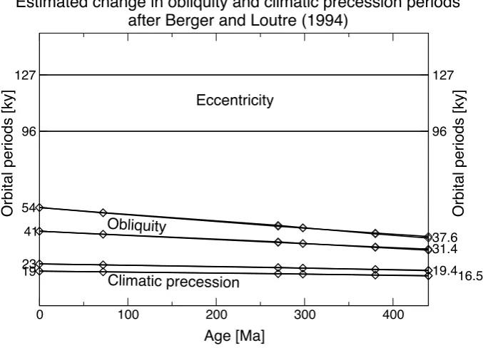
0 100 200 300 400

Age [Ma]

19 23

41 54 96 127

Orbital periods [ky]

16.5 19.4 31.4 37.6 96 127

Orbital periods [ky]

Eccentricity

Obliquity

Climatic precession

Estimated change in obliquity and climatic precession periods after Berger and Loutre (1994)

Figure 1.6: Estimated changes in the obliquity and climatic precession periods related to a changing Earth-Moon distance over the last 440 My, according to Berger

et al.(1989) [95], and Berger and Loutre (1994) [96]. Note that the periods of obliquity and climatic precession change due to a change of the precession constantp, while the eccentricity periods remain unaffected. Note that this figure is for illustrative purposes only, as the exact variation of orbital fre-quencies over tens of millions of years is not yet known in detail.

in the Earth’s rotational velocity leads to a redistribution of mass