Problem Data Based Optimization (PDBO)
Algorithm for Continuous Optimization Problems
Abdulelah G. Saif, Safia Abbas, and Zaki Fayed,
Member, IAENG
Abstract—Problem Data-Based Optimization (PDBO)
algorithm is appeared in 2015 by Abdulelah Saif, Safia Abbas and Zaki Fayed for combinatorial optimization problems and is applied to Discrete Time, Cost and Quality Trade -off problem (DTCQTP). In this paper, Problem Data-Based Optimization (PDBO) algorithm is adapted to solve continuous optimization problems. The proposed algorithm called the PDBO-CO (PDBO for continuous optimization) is tested on few benchmark functions and on COCOMO II model coefficients by using NASA 93 Dataset. The obtained results for benchmark functions are
compared with the ones obtained using
IWD-CO(Intelligent Water Drops for continuous optimization ) and the obtained results from the optimized COCOMO II PA model coefficients by PDBO-CO are compared with ones optimized by IWD and Genetic algorithm (GA) and with the current COCOMO II PA model coefficients. The obtained results are satisfactory, which encourage other researches in this regard.
Index Terms—COCOMO II, Meta-heuristic, Numerical functions, Optimization, PDBO algorithm
I. INTRODUCTION
PDBO algorithm is a single agent meta-heuristic algorithm that is invented for combinatorial optimization problems by applying it to DTCQTP which depends on possibility calculated from problem's data. PDBO assumes the problem is represented in the form of a graph G = (V, E), in which the set of nodes V represents the activities and modes, and the set of E represents edges that connects between activities and modes.
For optimization problems, at each iteration, PDBO selects the first node ni then depending on the best
possibility values, it moves to the next adjacent node nk.
After then, in order to increase the chance of selecting other nodes rather than node nk in the next iteration, PDBO
technique updates the Possibility(ni, nk) to be
Npossibility(ni,nk)=Possibility(ni, nk)+(cost/α) where α>0.
Finally, after the best iteration solution found, in order to evaporate the Npossibilities, PDBO considers the parameter β
[0,1], such that Npossibility(ni, nk)= Npossibility(ni, nk) Manuscript submitted July 23, 2015; revised July 29, 2015. The authors
gratefully acknowledge the support of Ain Shams University and Yemen government in supporting them.
Abdulelah Ghaleb Farhan Saif is Ph.D student at Ain Shams University, Egypt (phone: 00201154415035; [email protected]). Safia Abbas Mahmoed Abbas is lecturer at Ain Shams University, Egypt ( [email protected]).
Zaki Taha Ahmed Fayed is Emeritus Professor at Ain Shams University, Egypt ( [email protected]).
– β, where β is the evaporation rate (reduction rate) of Npossibility(ni, nk) for virtual edge between ni and nk[1].
The PDBO is single agent meta-heuristic. Meta-heuristics especially nature-inspired swarm-based optimization algorithms which are being increasingly used for solving optimization problems. Several meta-heuristics are basically suitable for continuous optimization whereas the rest of them are initially defined for combinatorial optimization. Particle swarm optimization [2] and ant colony optimization [3] are among the popular meta-heuristics, which are used for optimization problems.
So far, the PDBO algorithm has been used for the Discrete Time, Cost and Quality Trade -off problem (DTCQTP). Naturally, the PDBO algorithm is appropriate for combinatorial optimization problems. In this research, the PDBO is used for continuous optimization. In a continuous optimization problem, a number of continuous variables (parameters) are needed to be obtained such that a function is minimized or maximized. Here, the proposed PDBO algorithm called the “PDBO-CO” (the PDBO algorithm for continuous optimization) encodes the real continuous variables into integer numbers. Then, the PDBO tries to optimize the given function in the integer representation. Finally, the best solution is considered as the final solution. Next section talks about PDBO-CO. For this purpose, a few benchmark functions and COCOMO II model (for software cost estimation by using NASA 93 Dataset) are utilized for testing the proposed PDBO-CO for the continuous optimization, which are given in section III. At the end, conclusion is given in section IV.
II. THE PROPOSED PDBO-CO ALGORITHM
In this section, the steps to optimize a given function by the PDBO-CO are explained. In fact, solutions are constructed with the help of a graph. The proposed PDBO-CO is shown in figure 2. The following subsections explain the components of the PDBO-CO.
A. Problem Representation
Given a function f: S R, find X*
S:
X
S f(X*)
f(X) (minimization) or f(X*)
f(X) (maximization).Function f is called the objective function, its domain S is called the search space, and the elements of S, are called feasible solutions. A feasible solution X is a vector of optimization variables X = {X1, X2, ..., Xn}. A feasible
solution X*t hat minimizes/maximizes the objective function is called an optimal solution. The maximization over an objective function f is equivalent to minimization over the function –f [4].
Po
l
Po
Po
Po
Po
Po
Po
Po
..
l
..
..
...
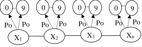
[image:2.595.49.284.151.229.2](digits i.e. domains) numbered from 0 to 9 which are connected to each node (variable) as in figure 1. Each of above variables is expressed by 4 digits which are chosen among 10 digits by PDBO_CO algorithm according to minimum possibilities (Po). First digit is integral part of a variable and the remaining 3 are fractions part. The possibilities are placed on the edges between variables and digits as in figure 1.
Fig. 1. Problem representation.
B. Possibilities Initialization
For each variable, X1,…,Xn, initialize the edges between
variable node Xi and its digits nodes Dk as follow:
Cost(Edge(Xi, Dk))=k, i=1,..,n, k=0,..,9 (1)
Calculate the total cost of Xi as
Total_Cost(Xi)=
9
0 k
k i
,
D
))
X
Cost(Edge(
, i=,1.,.n (2)E.g. Total_Cost(X1)=
9
0 k
k 1
,
D
))
X
Cost(Edge(
=Cost(Edge(1,0))+ Cost(Edge (1,1))+ …+ Cost(Edge(1,9)).
= 0+1+….+9=45.
Then, calculate the possibility of choosing the digit node Dk connected to variable node Xi among others as follow:
Possibility(Xi, Dk)=
)
(X
Total_Cost
))
D
,
X
Cost(Edge(
i k i
,where i=1,..,n, k=0,..,9 (3) E.g. Possibility (X1, D0)=0/45=0.0,
Possibility (X1, D1)=1/45≈0.022,
Possibility (X1, D2)=2/45≈0.044,
Possibility (X1, D3)=3/45≈0.066,
Possibility (X1, D4)=4/45≈0.088,
:
Possibility (Xn, D9)=9/45≈0.2.
C. Digit Selection Mechanism
PDBO_CO starts its journey from node1 (X1) from which
selects 4 digits among 10 digits which are connected to it according to minimum Possibility(X1,Dk) in order and
finishes it by visiting the last node (Xn) from which selects 4
digits among 10 digits which are connected to it. This step applies for all variables, if there is an improvement in the objective function, otherwise PDBO_CO selects four digits randomly from [0,9].
The 4 digits for each variable Xi are selected as follow:
Xi= 4 digits whose Possibility(Xi,Dk) are the smallest ,
i=1,….,n, k=0,…,9 (4) E.g. X1= 0123(four digits); these digits are selected by
PDBO_CO because 0.0, 0.022, 0.044 and 0.066 are the four smallest Possibility(X1,Dk) among all in order.
Note: You can make PDBO-CO selects more than 4 digits, if you need. To obtain negative value to variable, its selected digits are multiplied by -1.
D. Updates Possibilities
PDBO_CO updates the Possibility(Xi,Dk) of the four
selected digits for each variable Xi to be:
Possibility(Xi,Dk)=
Possibility(Xi,Dk)+
Dk))
Xi,
Cost(Edge(
(5)
,where α>0 (α user selected, here α=10000 ).
E. Evaporate Possibilities
In this step, PDBO_CO has two choices:
1. Evaporates the Possibility(Xi,Dk) of the four
selected digits for each variable Xi in the current
iteration, if there is an improvement in the objective function in the current iteration. 2. Evaporates the Possibility(Xi,Dk)of the best
selected digits for each variable Xi obtained
from all iterations ,if there is no improvement in the objective function in the current iteration. The equation used is:
Possibility(Xi,Dk)= Possibility(Xi,Dk)- β (6)
,where β >0 (β user selected, here β =0.00001).
1. Set α and β parameters.
2. Represent the problem in the form of graph as figure 1. 3. Determine problem dataset if exists.
4. Initialize the Possibility(Xi,Dk) , i=1,..,n, k=0,..,9.
5. While (termination condition not met) do For each variable Xi
if there is an improvement in the objective function then
Select 4 digits for variable Xi in the graph
with Minimum Possibility in order. Else
Selects 4 digits for Xi randomly from [0,9].
End if
Update Possibility of virtual edge between Xi and selected digit Dk by
Possibility(Xi,Dk)= Possibility(Xi,Dk)+
Cost(Edge(Xi, Dk))/α.
End i for
6. Find iteration solution i.e. evaluate the objective function.
7. If there is an improvement in the objective function then
evaporate the possibilities of virtual edges edge(Xi,
Dk) between all variables and their selected digits
at this iteration by Possibility(Xi,Dk)=
Possibility(Xi,Dk)- β.
Else
evaporate the possibilities of virtual edges edge(Xi,Dk) between all variables and their best
selected digits from all iterations by Possibility(Xi,Dk)= Possibility(Xi,Dk)- β.
8. End if 9. End while
10. Return the best solution
Fig. 2. The proposed PDBO-CO algorithm.
X
19
0
0
9
0
9
0
9
III. EXPERIMENTAL RESULTS
To evaluate the performance of the proposed PDBO-CO, a few benchmark functions taken from [5] and COCOMO II Post Architecture model [6] are selected. The algorithm is implemented in c# and is tested and evaluated on CPU (Core( i5) 3210 M, 2.50 GHz) and 4GB RAM using Windows 7 as the operating system.
A. Benchmark Functions
The selected functions are shown in table I. For the functions f1 , f2, f3 , and f4 , the dimension of the input vectors are here selected to be ten. In contrast, the dimension of the last function f18 is originally fixed to the value of two.
TABLE I:THE BENCHMARK FUNCTIONS, WHICH ARE USED FOR TESTING THE
PDBO-CO ALGORITHM
For each function, the PDBO-CO is run five times and the results are compared with that of IWD-CO found in [7]. The results of PDBO-CO and IWD-CO are shown in table II. The PDBO-CO converges to optimal values of the five functions.
TABLE II.THE RESULTS OF THE PDBO-CO AND IWD-CO Benchmark
function
PDBO-CO IWD-CO
Best value Average value Time (seconds) Best value Average value Time (seconds)
1 0 0 00.001000
0 1.28E-17 6.44E-16 68
2 0 0 00.006000
0 2.33E-08 3.92E -08 68
3 0 0 00.006000
4 2.09E-13 7.51E-11 65
4 0 0 00.001000
1 1.00E-06 2.25E -03 60
18 3.00025190 523812 3.20835 1 00.296016 9 3.00E+ 00
3.0000e 22
B. COCOMO II Post Architecture model
COCOMO II PA model is one of software cost estimation methods which calculates the software development effort (in person months) by using the following equation:
Effort = A × (SIZE)E ×
17
1 i
EMi. (7)
A- multiplicative constant with value 2.94 that scales the effort according to specific project conditions. Size - Estimated size of a project in Kilo Source Lines of Code or Unadjusted Function Points. E - An exponential factor that accounts for the relative economies or diseconomies of scale encountered as a software project increases its size. EMi - Effort Multipliers. The coefficient E is determined by weighing the predefined scale factors (SFi) and summing them using following equation:
E = B + 0.01×
5
1 i
SFi (8)
The development time (TDEV) is derived from the effort according to the following equation:
TDEV = C × (Effort)F (9)
F = D + 0.002 ×
5
1 i
SFi (10)
B=0.91,D=0.28. The values of effort multipliers and scale factors used in the implementation are taken from [6].
C. Dataset Description Used To Evaluate COCOMO
II PA Model
Experiments have been conducted on NASA 93 data set found in [8]. The dataset consist of 93 completed projects with its size in kilo line of code (KLOC), actual effort in person-month, development time in months .
IV. RESULT ANALYSIS
The best results of PDBO-CO, IWD[9] and GA [6] are achieved using many iterations and a solution set is received from which the best solution is chosen i.e. a solution with the best fitness function values (Mean Magnitude of Relative
Error (MMRE) for effort and time).
The final best solution obtained for coefficients(variables) by PDBO-CO is: A= 3.734, B=1.006, C=04.02 and D=0.327.
The final best solution obtained for coefficients(variables) by IWD is: A=3.762, B=1.005, C=4.484 and D=0.288.
The final best solution obtained for coefficients(variables) by GA is: A=3.673, B=1.005, C=02.44 and D=0.342.
Current COCOMO II PA model coefficients are the following: A=2.94, B=0.91, C=3.67 and D=0.28.
Benchmark Function Ranges Dim. Minimum value (fmin)
1 0 2)
(
1
n i ix
X
f
-5.12
xi
5.12 n
1 0|
|
|
|
)
(
2
1 0 1 0
n i i n i ix
x
X
f
-10
xi
10 n
1 02 1
0 0
)
(
3
n i i j jx
X
f
-100
xi
100 n
1 0n
i
x
X
f
i
0
|,
|
max
)
(
4
-100
xi
100 n
1 0)]
27
36
84
12
32
18
(
)
3
2
(
30
[
)]
3
6
14
3
14
19
(
)
1
(
1
[
)
(
18
2 2 2 1 2 2 1 1 2 2 1 2 2 2 1 2 2 1 1 2 2 1x
x
x
x
x
x
x
x
x
x
x
x
x
x
x
x
X
f
-2
xi
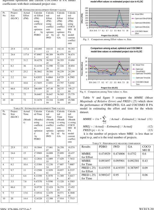
2The following tables, table III and table IV, show the comparison among the actual, effort and time, values and estimated, effort (person month) and time (months), values for the first ten project dataset using PDBO, IWD and GA algorithm optimized and current COCOMO II PA model coefficients with their estimated project size.
TABLE III: ESTIMATED DEVELOPMENT EFFORT VALUES
Pr. No Project Size (KLOC) Actual Effort (PM) Calculat ed Effort (PM) using coefficie nts optimize d by PDBO Calcula ted Effort (PM) using coeffici ents optimiz ed by IWD Calcula ted Effort (PM) using coeffici ents optimiz ed by GA Calcula ted Effort (PM) using COCO MO II PA model current coeffici ents
1 25.9 117.6 103.095 7 103.53 13 102.10 4 59.393 19 2 24.6 117.6 97.8907
3 98.309 42 96.979 11 56.674 13 3 7.7 31.2 30.4278 30.593
45
30.355 25
19.694 3 4 8.2 36 32.4158
6 32.590 29 32.326 37 20.854 73 5 9.7 25.2 38.3842
7 38.584 33 38.239 73 24.299 43 6 2.2 8.4 8.62855
5 8.6864 06 8.6729 28 6.2985 2 7 3.5 10.8 13.7655
4 13.851 4 13.797 84 9.6102 75 8 66.6 352.8 266.609
7 267.48 35 262.55 32 140.27 99 9 7.5 72 36.6467 36.847
18
36.565 1
23.779 46 10 20 72 33.1678
3 33.316 59 32.899 79 19.588 05
TABLE IV: ESTIMATED DEVELOPMENT TIME VALUES
Pr. No Project Size (KLOC) Actual Time (Month s) Calculat ed Time (Months) using coefficie nts optimize d by PDBO Calcula ted Time (Month s) using coeffici ents optimiz ed by IWD Calcula ted Time (Month s) using coeffici ents optimiz ed by GA Calcula ted Time (Month s) using COCO MO II PA model current coeffici ents
1 25.9 15.3 18.3044 1 17.061 07 26.358 58 10.574 9 2 24.6 15 17.9969
4 16.808 66 25.899 75 10.437 05 3 7.7 10.1 12.2816
2 12.009 55 17.429 3 7.7632 8 4 8.2 10.4 12.5384
5 12.230 24 17.807 27 7.8887 31 5 9.7 11 13.2508
6 12.839 61 18.857 14 8.2337 34 6 2.2 6.6 8.13350
6 8.3570 22 11.369 8 5.6417 87 7 3.5 7.8 9.47570
4 9.5590 73 13.320 3 6.3503 25 8 66.6 21 24.9739
6 22.424 72 36.374 03 13.452 05 9 7.5 13.6 13.0516
5 12.670 39 18.571 38 8.1840 16 10 20 14.4 12.6328
3 12.308 12 17.914 35 7.7515 3
The graphical comparison among effort values and among time values described in table III and table IV ,respectively is shown in figure 3 and figure 4 respectively.
Comparison among actual, optimizd and COCOMO II model effort values vs estimated project size in KLOC
0 50 100 150 200 250 300 350 400
25.9 24.6 7.7 8.2 9.7 2.2 3.5 66.6 7.5 20
Progect Size (KLOC)
E ff ort ( P M
) Actual Effort
Optimized Effort(PDBO)
Optimized Effort(IWD)
Optimized Effort(GA)
COCOMO II Model Effort
Fig. 3. Comparison among Effort values vs. Size.
Comparison among actual, optimizd and COCOMO II model time values vs estimated project size in KLOC
0 5 10 15 20 25 30
25.9 24.6 7.7 8.2 9.7 2.2 3.5 66.6 7.5 20
Progect Size (KLOC)
Ti m e ( M on ths ) Actual Time Optimized Time(PDBO) Optimized Time(IWD) Optimized Time(GA) COCOMO II Model Time
Fig. 4. Comparison among Time values vs. Size.
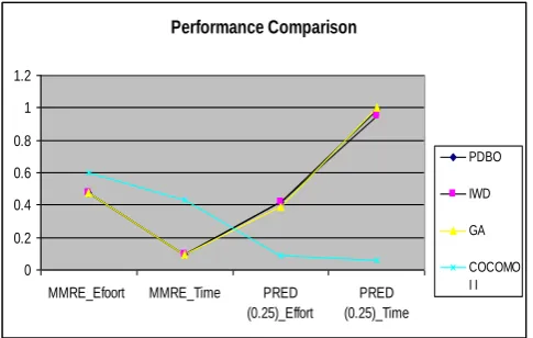
Table V and figure 5 compare the MMRE (Mean
Magnitude of Relative Error) and PRED (.25) which show
the performance of PDBO,IWD, GA and COCOMO II PA model in estimating the effort and time for the whole dataset.
MMRE = 1/n *
n
[image:4.595.38.552.116.815.2]j 1
| Actual – Estimated | / Actual (11)
MREj = | Actualj – Estimatedj | / Actualj (12) PRED (p) = k / n (13) k is the number of projects where MRE is less than or equal to p, and n is the total number of projects.
TABLE V: PERFORMANCE MEASURE COMPARISON
Results PDBO IWD GA COCO
MO II MMRE
for Effort
0.474929 0.474806 0.4752 0.6
MMRE for Time
0.093497 0.095901 0.092301 0.43
PRED (.25) for Effort
0.419355 0.419355 0.387097 0.09
PRED (.25) for Time
Performance Comparison
0 0.2 0.4 0.6 0.8 1 1.2
MMRE_Efoort MMRE_Time PRED
(0.25)_Effort
PRED (0.25)_Time
PDBO
IWD
GA
[image:5.595.48.291.52.206.2]COCOMO I I
Fig. 5. Performance measure comparison.
From table V and figure 5, the MMRE of PDBO, IWD and GA for effort and time is equal and lower than that of COCOMO II PA model ,whereas PRED(0.25) of PDBO and of IWD for effort is equal and for time PDBO is larger than that of IWD. PRED(0.25) of GA for effort is smaller than that of PDBO and IWD, but is the largest for time. COCOMO II is the worst among all.
It shows clearly that optimized coefficients by PDBO, IWD and GA algorithm produces more accurate results than the old coefficients.
V. CONCLUSION
This paper adapts PDBO algorithm to solve continuous optimization problems. The proposed PDBO algorithm, PDBO-CO, is tested on few well known benchmark functions and on COCOMO II PA model coefficients by using NASA 93 dataset. The obtained results for benchmark functions are compared with the ones obtained using IWD-CO and the obtained results from the optimized IWD-COIWD-COMO II PA model coefficients by PDBO-CO are compared with ones optimized by IWD and GA and with the current COCOMO II PA model coefficients. The obtained results aresatisfactory. In the future, other coding methods may be used instead of integer numbers.
REFERENCES
[1] Abdulelah G. Saif, Safia Abbas and Zaki Fayed, “The PDBO Algorithm for Discrete Time, Cost and Quality Trade -off in Software Projects with Expressing Quality by Defects”, to be published in Proceedings of International Conference on Communication, Management and Information Technology (ICCMIT 2015).
[2] Kennedy and Eberhart, “Particle Swarm Optimization”, Proceedings of IEEE International Conference on Neural Networks, Piscataway, NJ. (1995) 1942-1948.
[3] M. Dorigo, M. Birattari and T. Stuzle, “Ant Colony Optimization, Artificial Ants as a Computational Intelligence Technique”, IEEE Computational Intelligence Magazine, November 2006.
[4] Krzysztof Socha, “Ant Colony Optimization for Continuous and Mixed-Variable Domains”.
[5] Yao, X. and Liu Y, “Fast evolutionary programming ” In L. J. Fogel, P. J. Angeline & T. Back (Eds.), Proceedings of the 5th Annual Conference on Evolutionary Programming (pp. 451–460). SanDiego, CA: MIT Press.
[6] Astha Dhiman, Chander Diwaker, “Optimization of COCOMO II Effort Estimation using Genetic Algorithm”, American International Journal of Research in Science, Technology, Engineering & Mathematics, 2013.
[7] Hamed Shah-Hosseini, “An approach to continuous optimization by the Intelligent Water Drops algorithm”, 4th International Conference of Cognitive Science (ICCS 2011).
[8] Nasa 93 dataset contains effort and defect information available at
http://promisedata.googlecode.com/svn/trunk/effort/nasa93-dem/nasa93-dem.arff.
[9] Abdulelah G. Saif, Safia Abbas and Zaki Fayed, "Intelligent Water Drops (IWD) Algorithm for COCOMO II and COQUAMO Optimization", to be published.