Investigating the Polarization Tensor to Describe
and Identify Metallic Objects
Taufiq K. A. Khairuddin, Paul D. Ledger and William R. B. Lionheart
Abstract—This paper presents a few properties of the polar-ization tensor for conducting and magnetic objects to describe and classify the objects. In order to achieve this, the polarization tensor of the objects are numerically determined by the previous hp-FEM method. We then focus on the polarization tensor for magnetic but non-conducting objects. After that, the polariza-tion tensor for translated and rotated objects are discussed. Finally, this paper also highlights the polarization tensor for a few threat and non-threat objects which might appear in metal detection for security screening and landmine clearance.
Index Terms—metal detectors, land mine detection, eddy currents,hp-FEM method, matrices.
I. INTRODUCTION
I
N the eddy current approximation to Maxwell’s equation, Ammari et al. [1] derived an asymptotic formula that represented the perturbation of the magnetic fields due to the presence of an isolated conducting object. Two polarization tensors were then introduced from the formula, namely the conductivity polarization tensor (CPT) and the magnetic polarization tensor (MPT). They also designed a statistical algorithm to locate a spherical target based on induction data derived from eddy currents by using the CPT in [1] and extended it for an arbitrary target in [2].Furthermore, based on the foundation given in [1], Ledger and Lionheart [3] further investigated the MPT and CPT to describe conducting and magnetic objects. The reduction in the number of independent coefficients for the CPT and MPT for objects with rotational and mirror symmetries were also highlighted. They also applied tensor operations to introduce a new polarization tensor by combining MPT and CPT.
In the engineering literatures, Marsh et al. [4], [5] recon-structed the magnetic polarizability tensor of several detected objects by making measurements of the fields generated by the metal detector in order to describe the location, dimen-sion, orientation and material properties of an object for security screening. Similarly, Dekdouk et al. [6] conducted experiments to estimate the magnetic polarizability tensor of landmines to increase the chance of identifying them in a contaminated environmental field by using metal detector. It is shown in [3] that the magnetic polarizibilty tensor in [4], [5], [6] is the same as the rank 2 polarization tensor of [3] that combines both CPT and MPT.
In this study, the polarization tensor for a few objects are numerically computed according to the formula and method presented in [3].
Manuscript received March 13, 2015; revised April 9, 2015. This work was supported by the Ministry of Education of Malaysia and EPSRC under the grants EP/KO39865/1.
T. Khairuddin is with the School of Mathematics, The University of Manchester, UK and Department of Mathematical Sciences, Universiti Teknologi Malaysia, Johor Bharu, Malaysia. e-mail: ([email protected]).
P. Ledger is with the College of Engineering, Swansea University and W. Lionheart is with the School of Mathematics, The University of Manchester.
II. MATHEMATICALFORMULATION OF THE
POLARIZATIONTENSOR
The mathematical formulation of the polarization tensor is discussed now by considering first the eddy current model presented in [3]. Following Ammari et al. [1], we assume the presence of an object in the formBα=z+αB where Bis a unit object centered at the origin,αdenotes a scaling forB andzdenotes a translation vector. Introduce
µα= (
µ∗ inBα µ0 inR3\Bα
,σα= (
σ∗ inBα 0 inR3\Bα
(1)
whereµ0denotes the permeablitiy of free space while both µ∗ andσ∗ denote the permeability and conductivity of the
inclusion Bα. In this case, µ∗ and σ∗ are just constants
and we drop the subscript ∗ when considering B later on. Moreover, the conductivity contrast between the object and the background is assumed to be sufficiently high that the background can be approximated by a zero conductivity.
LetEα andHαbe the time harmonic eddy current fields (electric and magnetic) in the presence of conducting object Bα that result from a current sourceJ0located outside Bα. Suppose that∇·J0= 0inR3. Both fieldsEαandHαsatisfy the eddy current equations
∇ ×Eα=iωµαHαinR3, (2)
∇ ×Hα=σαEα+J0 inR3, (3)
Eα(x) =O(|x|−1), Hα(x) =O(|x|−1)as |x| → ∞ (4) where i is the standard imaginary unit andωis a fixed angular frequency of the current source. The depth of penetration of the magnetic field in the conducting object is desribed by its skin depth, s =p2/(ωµ0σ∗). On the other hand, without the objectBα, the fieldsE0 andH0that result from the time varying current source satisfy
∇ ×E0=iωµ0H0 inR3, (5)
∇ ×H0=J0 inR3, (6)
E0(x) =O(|x|−1), H0(x) =O(|x|−1)as |x| → ∞. (7) By introducing ν = 2α2/s2, the related asymptotic for-mula for the above model that describes the pertubation in the magnetic field at a position x, away from z, due to the presence of Bα when ν = O(1) and (µ∗/µ0) = O(1) as α→0is given by Ammari et al. [1] in the form
(Hα−H0)(x) =−iνα
3
2 P3
i=1H0(z)i( R
BD 2
xG(x,z)ξ×
(θi+ ˆei×ξ)dξ) +α3
1−µ0
µ∗
(P3
i=1H0(z)iD2xG(x,z)
R B eˆi+
1 2∇ ×θi
dξ) +R(x)
whereξis measured from the center of B. Here,G(x,z) = (4π|x−z|)−1is the free space Laplace Green’s function and
R(x) =O(α4)is a small remainder term. Furthermore, for i= 1,2,3,eˆiis a unit vector for thei-th Cartesian coordinate direction,H0(z)i denotes thei-th element of H0(z)i andθi is the solution to the transmission problem
∇ξ×µ−1∇ξ×θi
−iωσα2θi=iωσα2ˆei×ξ
inB∪Bc,
∇ξ·θi= 0 inBc,
[θi×nˆ]Γ=0 on Γ,
[µ−1∇
ξ×θi×nˆ]Γ=−2[µ−1]Γeˆi×nˆ on Γ,
θi(ξ) =O(|ξ|−1) as |ξ| → ∞ (9) wherenˆ is the outward normal vector toΓ, the boundary of B. Based on (8), two polarization tensors are introduced by [1] namely the conductivity polarization tensor (CPT) and the magnetic (permeability) polarization tensor (MPT).
Using this framework, Ledger and Lionheart [3] have applied tensor operations to combine both CPT and MPT as well as reformulate (8) in the alternative form
(Hα−H0)(x) =D2xG(x,z)MH0(z) +R(x) (10)
whereM is the new polarization tensor for a conducting and magnetic inclusion B. In their study [3], M is expressed either as rank 4 or rank 2 tensor. The hp-finite element method presented in [7] is also used in [3] to numerically compute M as both rank 4 and rank 2 tensors. For the purpose of this study, the same M as the rank 2 tensor is considered where our main motivation for choosing this is because it agrees with the engineering prediction about the polarization tensor for metal detector [3]. The rank 2 tensor M is given by [3] as
M =N−C (11)
where the coefficients of N andC are
α3
1−µ0
µ∗
Z
B
ˆ
el·ˆei+ 1
2eˆl· ∇ ×θi
dξ (12)
and
−iνα
3
4
ˆ
el· Z
B
ξ×(θi+ ˆei×ξ)dξ (13)
for l= 1,2,3.
III. METHODOLOGY
We now state several properties of the rank 2 tensor M. The coefficients ofM can be expressed as3×3matrix and it is proven in [3] thatM is complex symmetric so both real and complex parts ofM have three real eigenvalues. In their studies, [3] also explain that M =N for a magnetic non-conducting objectBα. Moreover,N here reduces to the first order Generalized Polarization Tensor (GPT) of [8] when Bα is simply connected andM can now be determined by solving boundary integral equations, which is given in [8] where the parameterkis the contrastµ∗/µ0 (or the relative permeability of Bα). In this case, an analytical formula of M for an ellipsoid is also given.
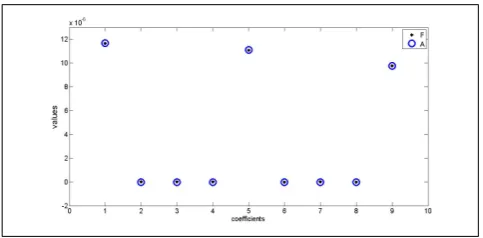
[image:2.595.306.548.51.170.2]Furthermore, M for an objectBα depends on the geom-etry, orientation and material of the object as given in (12) and (13). It also depends on the size but not on the position
Fig. 1. A comparison between the coefficients ofMfor a magnetic but non-conducting ellipsoid as obtained byhp-FEM method (F) and the analytical solution (A)
ofBα. In addition, if the objectBαis rotated and becomes Bα0, it can be shown by following [2] and [8] thatM forBα0 denoted byMB0 satisfies the following relation
MB0 =RMBRT (14)
whereMB is M for the original Bα,R is the appropriate rotation matrix andRT is the transpose ofR.
In this study, thehp-FEM method described in [3] is also used here to numerically computeM for a series of known objects relevant to magnetic induction such as in metal detector. The object is firstly approximated by a tetrahedral mesh by using the Netgen mesh generator [9] (see pictures in Table IV and Table V for examples). The mesh can be generated either as linear or quadratic elements and both are supported in the method. However, if the object has curved boundary segments, quadratic elements must be selected for the mesh. Here, the convergence ofM is achieved either by refining the size of the mesh inNetgen or by using higher degree polynomial of the edge element discretisation in the hp-FEM method.
IV. NUMERICALRESULTS
The polarization tensor M for magnetic non-conducting objects is firstly computed and presented in this section where the coeffiecients (elements) ofM in the first row are denoted starting from the first column by 1, 2 and 3 followed by 4, 5 and 6 for the second row, and 7, 8 and 9 for the third row. We then investigateM for a translated and rotated object. The polarization tensorM for a few threat and non-threat objects, which might appear in metal detection, are also considered.
A. M for Magnetic non Conducting Objects
LetBαbe the ellipsoid defined by x
2
a2+
y2 b2+
z2
c2 = 1where
a= 0.3,b= 0.2,c= 0.1centimeters (cm) and suppose that Bα is non-conducting and its relative permeability is equal to 1.5. By using 11665 tetrahedral meshes and polynomials of degree three in thehp-FEM method, an agreement of the computed coefficients ofM forBαto the analytical solution [8] is obtained. Figure 1 compares every coefficient ofM for Bα based on analytical solution given in [8] with the same coefficients ofM computed by thehp-FEM method.
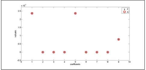
Fig. 2. A comparison between the coefficients ofM for a magnetic but non-conducting torus as obtained byhp-FEM method (F) and the boundary integral formulation of the first order GPT in BEM++ (A)
Fig. 3. The base of aL-shaped object
hp-FEM method. The diameter and height of the object are 0.2 and 0.1 cm, respectively, and the object has a cylindrical hole with diameter and height both approximately equal to 0.1 cm. Here, the convergence ofM in thehp-FEM method is achieved by approximating the object by 27919 tetrahedral meshes and uniformly increasing the degree of polynomial until order three. On the other hand, the boundary integral formula in [8] is numerically approximated by the software called as BEM++[10] which converges with 16174 surface elements.
B. M for a Translated and Rotated Object
In order to demonstrate the effect on the coefficients of the polarization tensor M under translation and rotation, we consider Bα as a three-dimensional L-shaped object (dimensions of the object are in cm). Here, the base of the object if viewed in two dimensions, is shown in Figure 3. Three pointsP,QandRare also chosen for references when translating or rotating the object.
We now assign the base to be above the xy-plane and for any point, p∈ Bα where (xp, yp, zp) is the coordinate of p in the three dimensional Cartesian coordinate system, xp, yp, zp≥0. We also let the height of the object to be equal to 1.5 so that 0 ≤ zp ≤ 1.5. In this case, P, Q and R are firstly set to be (0,0,0), (5.8,0,0) and (0,7.6,0) respectively. The object is approximated inNetgen by a linear mesh and assuming that the object is both conducting and magnetic (σ∗= 4.5×10⁶ S/m (Siemens per meter) andµ∗= 1.26×
10−4 NA−2 (Newton per ampere2)), the convergence of M for the object denoted by ML is obtained in the hp-FEM method by uniformly increasing the degree of polynomial until order three with 57456 tetrahedra. The convergedML
is written in the formML=R+Ji where
R= 10−3×
0.2314 −0.0818 0
−0.0818 0.3530 0
0 0 0.0686
(15)
and
J = 10−3×
−0.0200 0.0168 0 0.0168 −0.0400 0
0 0 −0.0024
. (16)
1) M for a translated object: In order to investigateM for theL-shaped object under a few translations, every point p that lies in the original object will be translated by a translation coordinatev= (vx, vy, vz) such that everypfor the translated object becomes (xp+vx, yp +vy, zp+vz). A fewv are considered, as listed in Table I, where the new P, Q,R as well as the new minimum and maximum values of zp are given. Each translated object is then created in Netgenand approximated by a linear tetrahedral mesh. Using these approximations,M for the object at every new position denoted byML0 is recomputed with thehp-FEM method. By
using the third order polynomial, eachML0 converges on the
mesh withNnumber of tetrahedra, where Nis also included in Table I.
Each ML0 is now compared with the original ML
where DL0 = ML0 −ML is firstly determined in the
software MATLAB. Let D˜L0 be a 9 × 1 column
vec-tor which contains all coefficients of DL0. By using the
function roundn in MATLAB, D˜L0 is round to 5 and
6 decimal places with the command roundn(D˜L0,−5)
and roundn(D˜L0,−6), respectively. The function any is
then applied to roundn(D˜L0,−5) and roundn(D˜L0,−6)
to decide whether D˜L0 is a zero column vector or not.
The outputs for commands any(roundn(D˜L0,−5)) and
any(roundn(D˜L0,−6)) in MATLAB are given as (d,−5)
and(d,−6) in the last two columns of Table I.
2) M for a rotated object: The L-shaped object at the original position in the Cartesian plane is now rotated three times. PointsP,QandRafter rotation as well as minimum and maximum value forzpof pointplying in the object, are given in Table II. The polarization tensorM for each object at the new position after rotation is denoted by MLr and computed after that. Similarly, each rotated object is firstly approximated by a linear tetrahedral mesh in Netgen. The number of elements N, needed for each MLr to converge after is computed by using the third order polynomial in the hp-FEM method are then given in Table II.
Next, the polarization tensor ML for the object at the original position is transformed three different times by using (14) according to each rotation performed to the object. The resulting transformedML is denoted byM˜Lr for each rota-tionr. The rotation matrixRused for each transformation is shown in Table III. EachM˜Lr is then compared to MLr by following the same steps as in the translation case.(dr,−5) and(dr,−6)in Table III are the results from MATLABthat tell whether a 9×1 column vector where its elements are all coefficients ofM˜Lr−MLr is a zero vector or not.
C. M for Threat and Non-threat Objects
TABLE I
TRANSLATION OF THEL-SHAPED OBJECT
Translation,L0 v P Q R zp(min) z
(max)
p N
(d, j)
j=−5 j=−6
1 (2,2,2) (2,2,2) (7.8,2,2) (2,9.6,2) 2 3.5 52993 0 1
2 (2,2,-2) (2,2,-2) (7.8,2,-2) (2,9.6,-2) -2 -0.5 55096 0 1 3 (-6,2,2) (-6,2,2) (-0.2,2,2) (-6,9.6,2) 2 3.5 55871 0 1 4 (-6,2,-2) (-6,2,-2) (-0.2,2,-2) (-6,9.6,-2) -2 -0.5 54844 0 1 5 (2,-8,2) (2,-8,2) (7.8,-8,2) (2,-0.4,2) 2 3.5 54242 0 1 6 (2,-8,-2) (2,-8,-2) (7.8,-8,-2) (2,-0.4,-2) -2 -0.5 51678 0 1 7 (-6,-8,2) (-6,-8,2) (-0.2,-8,2) (-6,-0.4,2) 2 3.5 53723 0 1 8 (-6,-8,-2) (-6,-8,-2) (-0.2,-8,-2) (-6,-0.4,-2) -2 -0.5 51248 0 1 9 (-1,-1,-0.5) (-1,-1,-0.5) (4.8,-1,-0.5) (-1,6.6,-0.5) -0.5 1 54918 0 1
TABLE II
ROTATION OF THEL-SHAPED OBJECT(A)
Rotation,r P Q R z(pmin) z(pmax) N
90◦aroundxy-plane (0,0,0) (0,-5.8,0) (7.6,0,0) 0 1.5 41583
90◦aroundxz-plane (0,0,0) (0,0,5.8) (0,7.6,0) 0 5.8 58648
90◦aroundyz-plane (0,0,0) (5.8,0,0) (0,0,7.6) 0 7.6 42358
TABLE III
ROTATION OF THEL-SHAPED OBJECT(B)
Rotation,r R (dr,−5) (dr,−6) 90◦aroundz-axis
0 −1 0
1 0 0
0 0 1
0 0
90◦aroundy-axis
0 0 −1
0 1 0
1 0 0
0 0
90◦aroundx-axis
1 0 0
0 0 −1
0 1 0
0 0
analogue (DA) of type 72 AP-mine [6] are categorized as threat objects. On the other hand, the following non-threat objects are considered : 1 pound British coin [12], a ball bearing (diameter 0.9 cm) and a belt buckle (see [11] for example). After choosing suitable values of ω for a metal detector and settingµ∗(NA−2) andσ∗ (S/m) for each object
according to its material,M for each object denoted byMB is computed by hp-FEM method. During all computations, after every object is approximated byNtetrahedral elements (mesh for both knife and gun are linear while others are quadratic), every convergedMB is obtained when the degree of the polynomial is increased uniformly to the third order in the hp-FEM method. Table IV and Table V shows the number of elements, N needed by MB for threat and non-threat object to converge.
In order to describe and identify each object, we first note that eachMB can be expressed asMB=RB+JBi where
RB andJBare real symmetric3×3matrices containing all real and complex coefficients ofMB, respectively. Two real symmetric3×3matricesMRBandMJB are now introduced where elements of MRB are absolute value of elements
(coefficients) of RB while elements of MJB are absolute value of elements of JB. Let ˆeMRB be a column vector
containing all normalized eigenvalues of MRB such that ˆ
eMRB contains every ratio of the eigenvalues ofMRB to the largest eigenvalues ofMRB. On the other hand, leteˆMJB be
a column vector containing every ratio of the eigenvalues of MJB to the largest eigenvalues ofMJB. We propose to use ˆ
eMRB andˆeMJB instead of the originalMB for describing
and identifying each object whereeˆMRB andˆeMJB are also
given in Table IV and Table V.
V. DISCUSSION ANDCONCLUSION
TABLE IV
THE NORMALIZED EIGENVALUES OFMFOR THREAT OBJECTS
Object,B Material N ˆeMRB eˆMJB
Knife stainless-steel 13621 1 1
µ∗= 1.26×10⁻⁶N A−2 0.9996 0.9355
σ∗= 1.39S/m 0.9957 0.0651
Gun type I steel 57456 1 1
µ∗= 1.26×10⁻⁴N A−2 0.4826 0.2113
σ∗= 4.50×10⁶ S/m 0.1741 0.0480
DA of 72 AP-mine aluminium 17257 1 1
µ∗= 1.26×10⁻⁶N A−2 0.3781 0.8578
σ∗= 3.50×10⁷ S/m 0.3781 0.8578
TABLE V
THE NORMALIZED EIGENVALUES OFMFOR NON-THREAT OBJECTS
Object Material N ˆeMRB eˆMJB
Belt Buckle titanium 32640 1 1
µ∗= 1.26×10⁻⁶N A−2 0.9995 0.0100
σ∗= 2.38×10⁶S/m 0.4170 0.0069
1 Pound Coin nickel-brass 23930 1 1
µ∗= 1.26×10⁻⁶N A−2 0.0083 0.0475
σ∗= 15.90×10⁶S/m 0.0083 0.0475
Ball Bearing type II steel 6252 1 1
µ∗= 4.40×10⁻⁴N A−2 1 1
σ∗= 4.65×10⁶S/m 1 1
them. In contrast to their works, polarization tensor for a few specified objects are numerically computed by solving (9) and using (11) in this study.
In order to provide numerical examples for this study, M for magnetic but non conducting objects are firstly considered. Since M in this case reduces to the first order GPT of Ammari and Kang [8] for simply connected objects, the accuracy of the computed M for the object can then
show excellent agreement betweenM computed by the given formula through hp-FEM method and the first order GPT. It can be seen that M for both ellipsoid and torus here are diagonal matrices. In addition, the first diagonal and the second diagonal entries ofM for the torus are equal.
Next,M for a translated and rotated object are examined. The three dimensional L-shaped object used here with the choosen µ∗ andσ∗ is actually the steel gun in Table IV. A
real situation is actually considered as our main motivation for this investigation where a person might carry a gun with many possible orientations on any part of his body when passing a metal detector during security checking. For this purpose, we first compute M for the object at a choosen initial position by using the hp-FEM method, resulting to the real and imaginary coefficients (15) and (16). The results show that M is complex symmetric as predicted by the theory in [3] for a conducting and magnetic object.
The results after 9 translations have been performed to the object are shown in Table I where the first eight of L0 move the object in each octant of the three dimensional space without including the origin. The lastL0translates the object from its initial position and lies within the intersection of every octant in three dimensional space, which will include the origin. M of the object at the original (initial) position is then compared to M for the object after it has been translated, which is also computed by thehp-FEM method. The values (d,−5) and(d,−6)in Table I are tests done in
MATLABto decide whetherD˜L0 is a zero column vector or
not after is rounded to 5 and 6 decimal places. If the value is 0 then D˜L0 is a zero column vector while 1 indicates
that D˜L0 has at least one non-zero element. In this case, for
eachL0,D˜L0 is a9×1zero column vector after is rounded
to 5 decimal places which implies DL0 =ML0−ML is a
zero matrix of size 3 and hence,ML0 =ML for allL0 at 5
decimal places or less, that isM of each translated object is the same asM of the object before translation. The results here consistent with our previous theory that M does not depend on the position of the object.
In addition, similar tests are performed in MATLAB to decide whether M of rotated objects computed by the hp -FEM method is similar to transforming M of the object at the original (initial) position according the same rotation. The results in Table II show that a column vector containing all coefficients ofM˜Lr−MLris a zero vector after is rounded to 5 and 6 decimal places. Consequently, at 6 decimal places or less,M˜Lr−MLr is a zero matrix of size 3 soM˜Lr =MLr for each r such that M of all rotated objects are similar to transformingM of the object at original position. These also give numerical evidences to suggest that M for the object at original position can be used directly to find M for the object after it is rotated, as given by (14). Therefore, it is then possible to identify an unknown object by reconstructing and comparing itsM to any transformedM for a known object. Finally, we also computeM for a few threat and non-threat objects in metal detection. A coin, a ball bearing of a toy (such as a yo-yo) and a belt buckle are non-threat objects during security check and coin also is a wanted object in treasure hunting by metal detector. Meanwhile, a gun and a knife are threat objects in security screening and a detonator analogue (DA) of type 72 AP-mine is the most important part in land mine detection. Here, the normalized eigenvalues
for real and imaginary parts ofM are used to describe all objects. Based on Table IV and Table V, we can see that ball bearing has one distinct normalized eigenvalues for both real and imaginary parts of itsM, coin and DA have two for each parts while others has three. Moreover, in contrast to other objects, DA and coin have the normalized eigenvalues of the imaginary parts to be either larger or equal to the normalized eigenvalues of the real part. This information is very useful to describe and classify the objects and can be further investigated. Our main aim after this will be to compare these results with the reconstructed polarization tensor and analyze them to hopefully improve metal detection in the future.
ACKNOWLEDGMENT
The authors were very grateful to Prof. Tony Peyton and Dr. Liam Marsh for their useful discussions on metal detec-tion and to Prof. Habib Ammari for his helpful suggesdetec-tions.
REFERENCES
[1] H. Ammari, J. Chen, Z. Chen, J. Garnier and D. Volkov, “Target detection and characterization from electromagnetic induction data,”
Journal de Math´ematiques Pures et Appliqu´ees,101, 54-75, 2014. [2] H. Ammari, J. Chen, Z. Chen, D. Volkov and H. Wang, “Detection and
classification from electromagnetic induction data,” submitted. [3] P. D. Ledger and W. R. B. Lionheart, “Characterising the shape and
material properties of hidden targets from magnetic induction data,” submitted.
[4] L. A. Marsh, C. Ktistis, A. J¨arvi, D. W. Armitage and A. J. Peyton, “Three-dimensional object location and inversion of the magnetic polarizability tensor at a single frequency using a walk-through metal detector,”Measurement Science and Technology,24(4), 2013. [5] L. A. Marsh, C. Ktistis, A. J¨arvi, D. W. Armitage and A. J. Peyton,
“Determination of the magnetic polarizability tensor and three dimen-sional object location for multiple objects using a walk-through metal detector,”Measurement Science and Technology,25(5), 2014. [6] B. Dekdouk, L. A. Marsh, D. W. Armitage, and A. J. Peyton,
“Es-timating magnetic polarizability tensor of buried metallic targets for landmine clearance,”Springer Science and Business Media, 425-432, LLC:2014.
[7] P. D. Ledger and S. Zaglmayr, “hp-Finite element simulation of three-dimensional eddy current problems on multiply connected domains,”
Computer Methods in Applied Mechanics and Engineering,199, 49-52, 2010.
[8] H. Ammari and H. Kang,Polarization and Moment Tensors : with Applications to Inverse Problems and Effective Medium Theory, Applied Mathematical Sciences Series,162, Springer-Verlag, New York, 2007. [9] J. Sch¨oberl “NETGEN : An advancing front 2D/3D-mesh generator
based on abstract rules,”Comput Visual Sci,1, 41-52, 1997. [10] W. ´Smigaj, S. Arridge, T. Betcke, J. Phillips and M. Schweiger,
“Solving boundary integral problems with BEM++,” to appear inACM Trans. Math. Software.