Hybrid Algorithm for Network Design Problem
with Uncertain Demands
Jan Roupec, Pavel Popela, Dusan Hrabec, Jan Novotny, Asmund Olstad, and Kjetil Haugen
Abstract—The purpose of the paper is to present a hybrid algorithm to solve a transportation optimization model with random demand parameters and network design variables. At first, the classical deterministic linear transportation model with network design 0-1 variables is introduced. Then, ran-domness is considered for demand parameters and modeled by here-and-now approach. The obtained scenario-based model leads to a mixed integer linear program (MILP) that can be solved by common integer programming techniques, see e.g. the branch-and-bound algorithm implemented in the CPLEX solver. Such a program may reach solvability limitations of MIP algorithms for large scale real world data, so a suitable heuristic development is welcome. Therefore, the idea of combination of traditional optimization algorithm and genetic algorithm is discussed and developed. At the end, the results are illustrated and also verified for a small test instance by figures.
Index Terms—transportation network-design problem, stochastic programming, scenarios, genetic algorithm, GAMS.
I. INTRODUCTION
T
HE paper introduces a hybrid solution technique for the scenario-based stochastic mixed integer linear program that models a design of transportation network under uncer-tain demand. Further useful references to basic concepts of stochastic programming can be found e.g. in [1] and [2].We start in Section II by considering a basic transportation network design problem, where the network connects sup-pliers and customers, see [3]. The presented transportation model is referred to as transportation model with adding edges (AE) throughout the paper.
In real-world problems, the costumer demand information can be unknown. This situation can be modeled by a stochas-tic programming here-and-now (HN) approach [1], which is the approach that we have adopted for the proposed paper. The stochastic version of the model is introduced in Section III and is called stochastic transportation model with AE.
Regarding the solution technique, we start off along our previous modeling ideas, see [4], but are eventually led to introduce a new hybrid algorithm to achieve the solution. The new solution techniques are discussed in Sections IV, V and VI. Selected results are shortly presented by illustrative figures – Section VII uses an artificial test case while Section VIII mentions the hybrid algorithm importance for the application area of waste-management network design.
We have to emphasize that the principal ideas of the introduced hybrid algorithm can be further applied to en-gineering optimization of design parameters. See [5], [6],
Manuscript received July 23, 2013; revised August 15, 2013.
J. Roupec is with the Institute of Informatics and Automation, FME, Brno University of Technology, 61669 Brno, Czech Republic, e-mail: [email protected]
P. Popela, D. Hrabec, and J. Novotn´y are with the Department of Statistics and Optimization, Institute of Mathematics, FME, Brno University of Technology, 61669 Brno, Czech Republic.
A. Olstad and K. Haugen are with Molde University College, Molde, Norway.
and [7] for civil engineering applications and [8], [9], and [10] for continuous casting, where both integer and continous variables may appear in the large scale instances of modeled problems. As we know, the model may involve linear and/or nonlinear terms, integer variables, and stochastic elements. Thus, the technique discussed in the paper may lead to further modifications of algorithms useful for modern en-gineering applications. In addition, the discussed heuristics can be modified with other algorithmic subroutines, see, e.g., [9], [11], and [12] for various possibilities.
II. TRANSPORTATION MODEL WITHAE
A transportation model, see [3], [13] and [14], is a first step towards our computations. The objective function is
max X
i1 X
e
Ai1,exe !
gi1− X
e
cexe− X
en
denδen (1)
and the goal is to maximize the profit. The following notation is utilized in the paper: Among decision variables, xe ≥0 is the amount of given product to be transported on edgee
and δen ∈ {0,1} is a 0-1 design variable, which is equal
to1 if a new edge en is built and0 otherwise. The sets of indices are:E is a set of edges, soe∈E , En is a set of newly built edges, soen∈En,I1 is a set of customers, so
i1∈I1,I2 is a set of plants (production places), soi2∈I2,
I3 is a set of transition nodes (no customer and no plant),
soi3∈I3, andI is a set of all nodes in a logistic network
that is i ∈ I =I1∪I2∪I3. Thus, Ai,e are elements of a network incidence matrix, where Ai,e = 1 if edge e leads to a node i. Ai,e = −1 if edge e stems from node i and
Ai,e = 0 otherwise. Additionally,gi1 is a unit selling price
for customeri1,ceis a unit transportation cost on edgee,den
is a cost of building a new edgeen, andbi are all demands
∀i∈I.
Then, the term P i1(
P
eAi1,exe)gi1 defines the income
from all customers. The next termsP
ecexe+Pendenδen
define the cost of transportation of produced items and setting up new edges in the network. The considered model is balanced i.e. the sum of demands is equal to the sum of produced and transported units of goods. This is also rep-resented by transportation balance constraintsP
eAi,exe=
bi,∀i∈I. So, the first model is then specified as follows maxP
i1( P
eAi1,exe)gi1− P
ecexe− P
endenδen
P
eAi,exe = bi, ∀i∈I,
xen ≤ δen(
P
i2−bi2), ∀en ∈En,
xe ≥ 0, ∀e∈E,
δen ∈ {0,1}, ∀en ∈En.
(2)
In the following step, we assume uncertain demand pa-rameters that we denote bi1,s,∀i1 ∈ I1, s ∈ S where
a finite number of realizations called scenarios denoted by indicess∈S. See also [4] for another model generalization involving pricing.
III. STOCHASTIC TRANSPORTATION MODEL WITHAE
Firstly, to include uncertainty in model (2), we utilize the HN approach and modify the objective function by a penalty term representing the expected penalty for the unsatisfied demand that is specified by new decision variablesyi+
1,s ≥0
andy−i
1,s≥0. So, we subtract formula P
sps( P
i1(q − i1y
− i1,s+
q+i
1y
+
i1,s)), which represents an additional cost, from the
objective function in model (2).
We also modify the first constraint from the model (2) as follows
X
e
Ai1,exe+y
+
i1,s−y −
i1,s=bi1,s, ∀i1∈I1,∀s∈S, (3)
where the equation (3) means that the transported units plus missing units minus surplus units must be equal to the customer demand. The following equations (4) and (5) are defined in the same way as in the model (2) but they are defined separately for plants (4) and for transition nodes (5).
P
eAi2,exe=bi2, ∀i2∈I2, (4) P
eAi3,exe=bi3, ∀i3∈I3. (5)
The new set of indices S is a set of all possible scenarios,
s ∈ S. So, the new decision variables are yi+1,s denoting a number of undertransported units i.e. y+i
1,s = bi1,s−xe
if bi1,s ≥ xe and is equal to 0 otherwise. Then, y − i1,s is a
number of overtransported units i.e.yi−
1,s=xe−bi1,s ifxe≥
bi1,s and is equal to 0 otherwise. Then, ps is a probability
of scenario s ∈ S, so 0 ≤ps ≤1,∀s ∈ S,Ps∈Sps = 1,
q+i
1 is a unit penalty for unsatisfied demand of the customer
i1 ∈I1,q−i1 is a penalty for transporting of redundant units
to customer i1 ∈ I1. New parameters are bi1,s number of
demand units by customer i1 ∈ I1, s ∈ S, bi2 number of
demand units by plant i2 ∈ I2 i.e. −bi2 is a number of
produced units by planti2∈I2,bi3= 0, i3∈I3. In total,bi
describes all demands and productions∀i∈I. Altogether we specify the updated scenario-based stochastic mixed-integer linear programming model as follows
maxP i1(
P
eAi1,exe)gi1− P
ecexe−Pendenδen−
P sps(
P i1(q
− i1y
− i1,s+q
+
i1y
+
i1,s)) P
eAi1,exe = bi1,s−y
+
i1,s+y −
i1,s, ∀i1∈I1,
∀s∈S,
P
eAi2,exe = bi2, ∀i2∈I2, P
eAi3,exe = bi3, ∀i3∈I3,
xen ≤ δen
P
i2(−bi2), ∀en ∈En,
yi+
1,s ≤ bi1,s, ∀i1∈I1,
∀s∈S, xe ≥ 0, ∀e∈E,
δen ∈ {0,1}, ∀en ∈En,
y+i1,s, yi−1,s ≥ 0, ∀i1∈I1, ∀s∈S.
(6)
IV. SOLUTIONALGORITHMS
We have implemented the aforementioned models (2) and (6) in GAMS and we have solved them by the use of CPLEX solver for small test instances obtaining acceptable results.
The next solution attempts to solve larger test problems in the same way led to significantly increasing computational time needs. Thus, we have decided to utilize our previous experience (see e.g. [15] and [16]) and we have developed a hybrid computational technique that combines the GAMS code with a selected genetic algorithm (GA). The flexible C++ implementation focusing on GAMS-GA interface fea-tures is set up for the modified GA that was discussed in [17], however, it is well suited also for other GA that can be linked and tested in the future, see, e.g. [18] or [19]. The following scheme is significantly inspired by the paper [16] that authors published with Jan Holesovsky in 2013.
Hybrid Algorithm
1) Set up the scenario-based GAMS model (read model and data in *.gms files). Set up control parameters for the GA. They are partly decided by the user (e.g. the population size) and partly inferred from the GAMS model counterpart (e.g. how many arcs in the network should be considered).
2) Create an initial population for the GA. Initial values of 0−1 variables must be generated and placed into the so called$INCLUDEfiles, where they can be read-in by GAMS. Several runs of random generation are needed, corresponding to the population size.
3) Repeatedly run (in parallel) tha GAMS model using tha CPLEX solver. Each run solves the program for the fixed values of0−1variables. Cost function values are calculated, also for new individuals created by means of the genetic operators, initially in 2. and then in 7. 4) Store the best results obtained from GAMS in 3. (the
optimal objective function values and optimal values of all variables) for comparisons.
5) Test the algorithm termination rules and stop in case of their satisfaction (e.g. after a long period of com-putations without any significant improvement in the objective function). Otherwise continue.
6) Generate input values for the GA from GAMS results, see step 3. Specifically, the cost function values for each member of population of the GA are obtained from results of the GAMS runs in 3.
7) Run GA to update the set of0−1 variables (popula-tion), see [17] for details. Return to step 3.
V. GENETICALGORITHMS
The section brings principal ideas of the utilized genetic algorithm (GA) that works as the principal part of the hybrid algorithm, see Section IV. It follows the previous ideas of one of the authors from [20] and [17] and brings much more details then the overview in [16].
Genetic algorithms belong to stochastic heuristic opti-mization methods, see [21]. GAs are inspired by biological mechanisms in a simplified way and they are implemented by computer codes. The main usage of GAs is the solution of problems of multi-dimensional optimization where no analytic or convergent numerical solution is known or is not achievable.
find the best one (full enumeration technique). However, in theoretical models, the feasible set is usually an infinite set because of continuous decision variables. Even in practice, such procedure is not often useful although when we use a computer, the feasible set can be considered finite because we cannot store infinite set of numbers in the finite memory. Yet in real-world problems we cannot explore all possible values of the objective function in the time that is available. So, heuristic methods use more advanced strategies.
The feasible set search strategy used by GAs is inspired by natural evolution, where the best individuals have the best chance to survive and to become parents of new offspring. GA has an iterative character. GA works not only with one solution in time but with the whole population of solutions. The population contains many (often several hundreds) indi-viduals i.e. bit strings representing solutions. The mechanism of GA involves only elementary bit related operations like strings copying, partially bit swapping or bit value changing. The GA begins with a population of strings and thereafter generates successive populations using the following three basic operations: reproduction, crossover, and mutation.
Reproduction is the process by which individual strings are selected as the parents of new offspring according to an objective function value (so called fitness). This means that strings with a higher fitness value have a higher probability of contributing one or more offspring to next generation. This is an artificial version of natural selection. Usually two parents are selected to create a new bit string - the new individual (child). The new bit string is created by a combination of parts of bit strings of its parents (the child inherits genetic information from its parents). This string combination is called crossover. These new children are added into the population. The population has the constant size, so it is necessary to delete some (almost all) parents (so called deletion operator). Then the process is repeated (i.e. next iteration runs) with the new population. If the stopping rule is satisfied, the process ends.
In addition, the GA utilizes another mechanism existing in the nature - mutation. Theory says that mutation helps individuals adapt to changing living conditions easier. It is modeled as a small random change of genetic information. Mutation is an occasional (with a small probability) random alteration of the string position value. Mutation is needed since, in spite of reproduction and crossover effectively searching and recombining the existing representations, they occasionally become overzealous and lose some potentially useful genetic material. The mutation operator prevents such an irrecoverable loss. The recombination mechanism allows mixing of parental information while passing it to their descendants, and mutation introduces innovation into the population. Mutation can also prevent degeneration. In opti-mization the deadlock in a local extreme is interpreted as an analogy to degeneration.
More details on GAs and its operators and parameters can be given as follows. There is a populationPcontainingN el-ements (individuals). Each element ofP is a string (or set) of integers of the fix length ofnrepresenting the solution of the problem. Then,f denotes the cost function (fitness function) which assigns a real number to each individual inP. There is a parent selection operator, which selects elements fromP. In general, we consider a set of genetic operators containing:
the crossover operator, the mutation operator, and eventually other problem dependent or implementation dependent oper-ators. All these operators generate descendants from parents. The parent selection operator and the genetic operators have the probabilistic character and the deletion operator is usually deterministic. Depending on implementation an individual contains one or more chromosomes. The genotype of chromosome is the inner representation of chromosome in the computer memory. Usually, the inner representation is treated as a vector of genes. The phenotype of chromosome is an abstract mathematical object representing the solution of solved optimization problem. We can treat it as a vector containing graph structure description, parameter values, etc. The use of computers is expected, so the chromosome is stored in the memory in the form of field of bits. This field must have the finite length. It means that the set of all possible phenotypes of chromosomes is finite too. The ambition of evolution is to create a chromosome, which is very near (or even equal) to the optimal chromosome. As mentioned above, the mutation and crossover operators have a probabilistic character, so we can denote the probability of mutation and probability of crossover. The fitness value
f is a non-negative number bringing a relative measure of the quality of every individual in the current population. The run of GA can be described using the following steps:
1) Generation of the initial population (random generation is often used) composed of individuals.
2) Computation of fitness function values related to 1). 3) Parent selection and generation of offspring.
4) Creation of the new population by using deletion operator and addition of offspring generated in the previous step.
5) Mutation.
6) If the stopping rule is not satisfied, go to step 3), otherwise continue to 7).
7) The result is the best individual in the population.
VI. IMPLEMENTATION DETAILS AND TRICKS
In spite of its simple principles, the design of the GA to be practically successful can be surprisingly complicated, see [17] and [20] for further details. The GA has many parameters that depend on the problem to be solved. In the first, it is the size of population. There are two opposite demands.
The diversity (the amount of information in the population) should be as high as possible. The speed of computations should be high and it depends on the number of computations in every iteration. Larger populations usually decrease the number of iterations needed but dramatically increase the computing time for each of iteration. The factors increasing demands on the size of population are the complexity of the problem being solved and the length of the individuals. A smaller population brings the problem of degeneration (premature stop of computations). The optimal size of popu-lation increases exponentially with the length of genes when binary coding is used. Practical experiences show that the population size of 50 – 200 produces usually good results in many cases, whereas for large problems up to 1000 individuals in population should be used.
genes. Genes are the elements of the parameters vector. The value represented by chromosome has to be decoded. To eliminate the influence of the Hammings barrier, Grey code must be usually used, see [21]. We can consider the gene to be a structure representing one bit of the solution value. It is usually advantageous to use some redundancy in genes and then the physical length of the genes can be greater than one bit. Such a type of redundancy was introduced by Ryan [22].
The so called shades mean that chromosomes contain redundant information every value bit is stored in one gene having length of more than one bit. E.g. for genes of the length of three bits gene values 0, 1, 2 could represent value 0, gene values 5, 6, 7 could represent value 1, and values 3 and 4 could be an undetermined (shade) area their value is set randomly (once for the whole lifetime of each gene).
The strategy of generation of the initial population is also important. Usually it is generated randomly, but we can also use solutions obtained by another methods (in this case we talk about hybrid GA). It is useful to reach a high diversity in the initial population, therefore using identical individuals in the initial population is not recommended.
There is also a significant problem with infeasible solu-tions. Usually, initial population should not contain infeasible solutions. Infeasible solutions can also appear as a product of the crossover and/or mutation operation. Such population members could be excluded from the population, but some-times it is more convenient to penalize them (by assigning a very poor value of the cost function to these individuals).
One of the most important details is the parent selection strategy. The diversity is dramatically decreased when only the best individuals are selected for crossover. Three basic strategies are used: (1) Proportionate selection – the prob-ability of selection of each individual is proportionate to its fitness. (2) Ranking selection – population is sorted by the fitness, the probability of selection of each individual is proportionate to its rank in population. (3) Tournament selection – several individuals are selected randomly, from them the individual with the best fitness is taken.
New individuals are created by operation called crossover. In the simplest case, crossover consists in swapping two parts of two chromosomes split in randomly selected point (the so-called one point crossover). It is also possible to use multi-point crossover. Depending on the application, the multi-point of crossover can be located inside the genes or only on their borders. Uniform crossover means that every gene (or even every bit) of the new individual is randomly chosen from one parent.
The main goal of mutation is to eliminate degeneration and to allow changes of genotype, which cannot be reached by crossover. There are different kinds of realization of mutation operation (to change one bit, a group of bits, to change one gene, arithmetic operation applied to a chosen element of vector of solution in chromosome,. . .). The mutation has a probabilistic character (bits/genes/chromosomes are selected randomly); the corresponding parameter is the probability of mutation.
The classical version of GA uses only three genetic oper-ators – crossover, mutation and reproduction (e.g. the parent selection and the replacement scheme). One of the biggest disadvantages is a tendency of GA to reach some local
ex-treme. In this case GA is often not able to abandon this local extreme in he consequence of the low variability of members of population. To prevent the degeneration and the deadlock in local extreme, a limited lifetime of individuals can be used. The limited lifetime is realized by the death operator [17], which represents something like a continual restart of the GA. This operator enables decreasing the population size as well as increasing the speed of convergence. Each individual carries an additional information its age. A simple counter, which is incremented in each iteration of the GA, represents the ageing. If the age of any member reaches the preset lifetime limit LT, the member dies and is immediately replaced by a new randomly generated population member. The age is neither mutated nor crossed over. The age of new individuals (incl. individuals created by crossover) is set to zero. A useful range for the lifetime limit is from 5 to 20, in dependence on the population size and the typical number of iterations. It is necessary to store the best obtained solution separately the corresponding individual might not always be present in the population because of the limited lifetime.
Many GAs are implemented on a population consisting of haploid individuals (each individual contains one chromo-some). However, in nature, many living organisms have more than one chromosome and there are mechanisms used to determine dominant genes. Sexual recombination generates an endless variety of genotype combination that increases the evolutionary potential of the population. Because it increases the variation among the offspring produced by an individual, it improves the change that some of them will be successful in varying and often-unpredictable environments they will encounter. The modeling of sexual reproduction is quite simple. The population is divided into two parts - males and females. One parent from each part is selected for crossover. The sex of individual is stored in the special gene; this gene is not mutated. The sex of descendant is determined by crossover the sexual genes of parents, descendant is placed to the corresponding part of population. There are different selection strategies of parent of different sex (analogies of biological systems are used).
the same. Newly created individuals of low fitness do not have to be involved in the population.
Genetic algorithms commonly use heuristic and stochastic approaches. From the theoretical viewpoint, the convergence of heuristic algorithms is not guaranteed for the most of application cases. That is why the definition of the stopping rule of the GA brings a new problem [23]. We must notice that a typical GA does not produce the solution enhancement in every iteration. The stagnation can be observed in follow-ing three situations: (1) Temporary stagnation, GA is able to continue. (2) Local extreme was reached and population is degenerated, GA is probably not able to continue. (3) The optimal solution was found (this solution is unknown, so this situation cannot be simply identified).
It can be shown that while using a proper version of GA repeatedly for the given problem, the typical number of iterations can be determined.
The hybrid algorithm described in the paper uses GA as the main control loop. The GA is implemented in C+ language in the object form. The computation of the objective function value is rather complicated in this case, so we de-cided not to write a C++ program to solve the network design problem, but use the GAMS with CPLEX solver instead. In opposite way, we have not fully utilized GAMS and CPLEX for the whole model to avoid a need to solve a large scale mixed integer program. The used approach advantageously splits the solution between GA and LP solver.
The communication between GA and GAMS is based on data transfer by external interface files. The time consump-tion for the cost funcconsump-tion evaluaconsump-tion in this arrangement is high. It was necessary to minimize the number of the cost function evaluation (the number of running GAMS). The very efficient version of GA capable to find solution in a small number of iterations and capable to use a small popu-lation was needed. The GA used in the paper problem related computations uses ranking selection, haploid chromosomes, shadows, limited lifetime and elitism described above.
The results for the test example were obtained by the GA having the population size of 40 individuals that can be computed in parallel to save a computational time. The typical number of iteration was about30, so the GAMS was called1200times in the worst case. The chromosomes have the length of 119 data bits, so more then 6.6×1035 of
combinations describing the feasible set exist (so the use of the full enumeration strategy is not definitely possible in this case).
VII. COMPUTATIONS ANDRESULTS
The main idea of the hybrid algorithm is based on the solution of a stochastic program for various sequences of the fixed0−1variables. So, the the optimal objective function values are obtained together with these sequences of zeros and ones. They serve as the input fitness value plus elements of the population for the GA that utilizes its own steps described below (selection, crossover, mutation and further modifications as limited lifetime and sexual recombinations, see [17]) that are hidden within the GA structure. Updated sequences of zeroes and ones are generated by the GA and sent to the GAMS through the updated$INCLUDEfile and the computational loop continues to the moment when the satisfactory improvement of the network design is obtained.
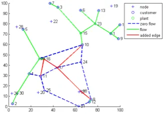
[image:5.595.344.508.133.261.2]Because of the comparison purposes, we have utilized the test examples from [4]. The results obtained by the hybrid algorithm seem to be equivalent to GAMS computations for the considered instances, see Figure 1 and 2 for the selected case.
Fig. 1. Results for the deterministic transportation model with AE.
Fig. 2. Results for the stochastic transportation model with AE.
The figures represent visualization of the example for main models, see [14] for details. The example shows a distribu-tion network (green lines are edges where the variablesxeare non-zeros, red lines are edges where xen is a non-zero one
(or δen is equal to1)). We may also see that the stochastic
demand usually requires new edges to bring the necessary recourse in the results.
VIII. CONCLUSIONS ANDFURTHERRESEARCH
The paper presents principle ideas behind the development of the original hybrid algorithm involving GA for the solution of network design problem (6). We have focused on a specific network design problem with uncertain demands leading to the large scale specially structured mixed integer mathematical program. Similar mixed integer programs may appear in many application areas, including traffic networks [16], design problems [6], and production problems [10]. Therefore, the suggested hybrid algorithm can be modified and widely applied. The similar hybrid algorithm technique has been already utilized for traffic assignment problem in [16]. The hybrid algorithm description is also accompanied by details about the implemented GA.
[image:5.595.344.510.316.432.2]In addition, the developed hybrid algorithm framework is general enough that allows to replace its elements, e.g. GAMS with other modelling language and the chosen GA with other GAs or heuristics. The approach is also portable to other problems leading to nonlinear integer programming formulations.
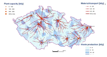
Fig. 3. Waste management network design - feasible edges.
Fig. 4. Waste management network design - suboptimal solution.
The idea to test these conclusions more carefully for large test cases and real world applications in waste management problems (see [24] for recent challenges), especially in the related transportation network design (see Figure 3 for visualised network and Figure 4 for achieved results by [25] with details) represents one of the current challenges for further research. Another challenge is to apply developed techniques in collaboration with colleagues specializing in traffic organization under uncertain or stress circumstances, see [16], [26], and [27]. In addition, we have to think about generalization of our hybrid technique to the transportation problems involving pricing as in [4].
ACKNOWLEDGMENT
The present work has been supported by European Re-gional Development Fund in the framework of the re-search project NETME Centre under the Operational Pro-gramme Research and Development for Innovation. Reg. Nr. CZ.1.05/2.1.00/01.0002, id code: ED0002/01/01, project name: NETME Centre -New Technologies for Mechanical Engineering and by FME BUT standard specific research project for 2013. The support from Strategiskhoyskole-prosjekt of Molde University College is also gratefully acknowledged.
REFERENCES
[1] A. Shapiro, D. Dentcheva, and A. Ruszczynski,Lectures on Stochastic Programming: Modeling and Theory. SIAM, 2009.
[2] J. Novotn´y,Stochastic programming models with applications. master thesis, FME, Brno University of Technology, Brno, CR, 2008. [3] G. Ghiani, G. Laporte, and R. Musmanno,Introduction to Logistic
Systems Planning and Control. John Wiley & Sons, 2004. [4] D. Hrabec, P. Popela, J. Novotn´y, K. K. Haugen, and A. Olstad, “The
stochastic network design problem with pricing,”In Proceedings of the 18th International Conference of Soft Computing MENDEL 2012, pp. 416–421, 2012.
[5] I. L´anikov´a, P. ˇStˇep´anek, and P. ˇSimunek, “The fully probabilistic design of concrete structures,”In Proceedings of the 16th International Conference on Soft Computing MENDEL 2010, pp. 426–433, 2010. [6] P. ˇStˇep´anek, J. Plˇsek, I. L´anikov´a, F. Girgle, and P. ˇSimunek,
“Op-timization of concrete structures design,”In Proceedings of the 16th International Conference on Soft Computing MENDEL 2010, pp. 434– 440, 2010.
[7] P. ˇStˇep´anek, J. Plˇsek, I. L´anikov´a, and P. ˇSimunek, “Life time assessment and deterministic based optimization of concrete structure design,”In Proceedings of the 17th International Conference on Soft Computing MENDEL 2011, pp. 301–306, 2011.
[8] T. Mauder, F. Kaviˇcka, J. ˇStˇetina, Z. Franˇek, and M. Masarik, “A mathematical stochastic modelling of the concasting of steel slabs,”In Proceedings of the 18th International Conference METAL 2009, pp. 41–48, 2009.
[9] T. Mauder, ˇC. ˇSandera, M. ˇSeda, and J. ˇStˇetina, “Optimization of quality of continuously cast steel slabs by using firefly algorithm,”In Proceedings of Conference on Materials and Technology, pp. 45–53, 2010.
[10] J. ˇStˇetina, L. Klimeˇs, T. Mauder, and F. Kaviˇcka, “Final-structure pre-diction of continuously cast billets,”Materiali in tehnologije, vol. 46, no. 2, pp. 155–160, 2012.
[11] R. Matouˇsek, “GAHC: Improved GA with HC mutation,” World Congress on Engineering and Computer Science WCECS 2007, pp. 915–920, 2007.
[12] R. Matouˇsek and E. ˇZampachov´a, “Promising GAHC and HC12 algorithms in global optimization tasks,” Optimization Methods & Software, vol. 26, no. 3, pp. 405–419, 2011.
[13] S. P. Bradley, A. C. Hax, and T. L. Magnati,Applied Mathematical Programming. Addison-Wesley, 1977.
[14] D. Hrabec,Stochastic Programming for Engineering Design. master thesis, FME, Brno University of Technology, Brno, Czech Republic, 2011.
[15] J. Roupec and P. Popela, “Genetic algorithms for scenario generation in stochastic programming: Motivation and general framework,”Lecture Notes in Electrical Engineering, vol. 14, pp. 527–536, 2008. [16] J. Holeˇsovsk´y, P. Popela, and J. Roupec, “On a disruption in congested
networks,”In Proceedings of the 18th International Conference of Soft Computing MENDEL 2013, accepted.
[17] J. Roupec, “Advanced genetic algorithms for engineering design problems,” Engineering Mechanics, vol. 17, no. 5-6, pp. 407–417, 2011.
[18] R. Matouˇsek, “HC12: The principle of CUDA implementation,”In Proceedings of the 16th International Conference on Soft Computing MENDEL 2010, pp. 303–308, 2010.
[19] ——, “HC12: GAHC improved genetic algorithm,”In Nature Inspired Cooperative Strategies for Optimization (NICSO 2007), 2007. [20] J. Roupec, Design of Genetic Algorithm for Optimization of Fuzzy
Controllers Parameters (In Czech). PhD thesis, Brno University of Technology, Brno, Czech Republic, 2001.
[21] D. E. Goldberg, Genetic Algorithms in Search, Optimization, and Machine Learning. Addison-Wesley, 1989.
[22] C. Ryan, “Shades: Polygenic inheritance scheme,”In Proceedings of the 3rd International Conference on Soft Computing MENDEL 1997, pp. 140–147, 1997.
[23] J. Roupec, P. Popela, and P. Osmera, “The additional stoping rule for heuristic algorithms,” In Proceedings of the 3rd International Conference on Soft Computing MENDEL 1997, pp. 135–139, 1997. [24] M. Pavlas, M. Touˇs, L. B´ebar, and P. Stehl´ık, “Waste to energy? an
evaluation of the environmental impact,”Applied Thermal Engineer-ing, vol. 30, no. 16, pp. 2326–2332, 2010.
[25] R. ˇSompl´ak, V. Proch´azka, M. Pavlas, and P. Popela, “The logistic model for decision making in waste management,” Chemical Engi-neering Transactions, vol. 35, 2013.
[26] J. Mazal, P. Stodola, and M. Podhorsk´y, “Traffic management opti-mization and its modeling,”Recent Advances in Energy, Environment and Economic Development, pp. 274–279, 2012.
[image:6.595.65.268.312.420.2]