On using Directional Information for Parameter Space Decomposition in Ellipse Detection

Pergamon

Pattern Recognition, Vol. 29, No. 3, pp. 369 381, 1996 Elsevier Science Ltd Pattern Recognition Society Printed in Great Britain. 0031-3203/96 $15.00 +.00

0031-3203(94)00096-8

ON USING DIRECTIONAL INFORMATION FOR PARAMETER

SPACE DECOMPOSITION IN ELLIPSE DETECTION

ALBERTO S. A G U A D O , M. E U G E N I A M O N T I E L and M A R K S. NIXON* Department of Electronics and Computer Science, University of Southampton, Highfield,

Southampton S017 I BJ, U.K.

(Received 19 January 1995; in revised form 5 June 1995; received for publication 3 July 1995)

Abstract--In this paper we use the parameteric polar representation to extend the application of edge directional information from circle to ellipse extraction. As a result we obtain a mapping which decomposes the parameter space required for ellipse extraction into two independent sub-spaces and one final histogram accumulator. The mapping includes the tangent of the angle of the first and second directional derivatives. These tangents are computed by considering edge direction at two border points. We show that the use of gradient information for parameter space decomposition avoids the intensive point labelling imposed by geometric constraints used by other approaches.

Computer vision Ellipse detection

Image segmentation Feature extraction Parameter space decomposition

Hough transform

l. I N T R O D U C T I O N

The detection of geometric primitives from an image is one of the basic tasks of computer vision. A geometric primitive is represented by a mathematical expression with a number of free parameters which define instan- ces of a shape. Hence, the extraction problem centres on obtaining an estimate of the free parameters ac- cording to the information on an image. The Hough transform (HT) is a well-known method to detect shapes by independently considering geometric data composed of edge points. The independent evidence accumulation of the HT makes it robust, providing adequate results even for overlapping or partially oc- cluded objects.

In order to gather evidence, the HT defines a map- ping from the image space into a parameter space. By considering each border point in an image, the map- ping adds a vote to chosen cells in an accumulator which represents the parameter space. The cells in- creased are those whose associated parameters define the geometric primitive which passes through the im- age point. Therefore, local maxima in the accumulator array correspond to the parameters of detected shapes. The HT was originally proposed to fit straight lines and then extended to analytical curves31~ Although the technique can be used directly for any parameterized curve, the generalization implies an exponential in- crease in computational time and space requirements. for this reason, new methods based on the original HT have been proposed (a review of the methods can be seen in Illingworth & Kittler ~2~ and Leaversta~).

* Author to whom correspondence should be addressed. © Crown copyright (1996).

The aim of this paper is to show how directional information can be used to derive a mapping which decomposes the parameter space required for the im- plementation of the HT. In addition to image points, we consider edge direction as geometric data provid- ing an important clue for evidence gathering in the parameter space.

Edge direction information has been used success- fully to reduce the computational requirements of the HT in circle extraction, ca'5) The general approach is to include gradient direction information in order to constrain the parameter space. Here we show how the parametric polar representation can be used to com- bine edge points and gradient direction information in order to establish an explicit analytic description of the mappings between the image and parameter spaces, which only involve a sub-set of the complete parameter set. We extend the ideas of circle parameter decompo- sition to ellipses by combining the para- metric polar form with the first- and second-order directional derivatives. This allows us to obtain two independent bi-dimensional sub-spaces, each of which relates two ellipse parameters. A final histogram accu- mulator is used to evaluate the remaining parameter.

Previous methods for ellipse extraction ~6-111 have shown that it is possible to reduce the dimensions of the parameter space by, using geometric properties of an ellipse. These properties involve geometric con- straints between edge points and are used to find expressions which relate only chosen ellipse para- meters. The geometric constraints include distance or angle relationships that define the relative position between a set of points. Hence, the parameters of an ellipse are computed after searching for edge points

which satisfy the constraints. The major difference between previous approaches and our approach is the consideration that two edge points define the ratio between directional derivatives, of first and second order, of the parametric polar functions of another point. The most important result of this paper is that the constraints, which define relative positions be- tween points (as required by other approaches), are avoided by taking only two points on an ellipse and the gradient direction information. In contrast to the polar representation~9,10) and the tangent representation of curves, ~8) the parametric polar representation ex- presses, in an explicit form, the relationship between the parameters of an ellipse and the directional deriva- tives. This is used to solve analytically the equations which decompose the parameter space.

This paper is organized as follows. In Section 2 we consider the parametric polar representation of an ellipse and its derivatives. In Section 3 we present the generalization of the two-plane HT for circles to ellips- es. It is shown that the use of the first directional derivative alone does not offer a computationally at- tractive result, making necessary the inclusion of the second directional derivative in an ellipse definition. In Section 4 we show how this information can be com- puted from geometric data on an image. Section 5 pres- ents the implementation and experimental results. In order to reduce accumulator noise for complex images, some considerations which prevent numerical impreci-

and their derivatives are defined by:

x(O) = a o + rcos(0), y(O) = b o + rsin(0),

x'(O) = - r sin(0), y'(O) = r cos(0), (1)

x"(O) = - r cos(0), y"(O) = - r sin(0),

where 0~(0,2n] and the parameters (ao, bo) are the coordinates of the circle's centre with radius r.

If a circle is scaled by choosing different values of r in the expressions for x(O) and y(O), then the curve corre- sponds to an ellipse:

x ( O ) = a o + a C o s ( O ) , y ( O ) = b o + b s i n ( O ), (2)

where a and b are the length of the axis in the x and y directions, respectively.

An additional parameter p defines the rotation of the ellipse with respect to the x axis. The locus of a rotated ellipse is then defined by (xp(O), yp(0)):

[-(xp(0)- ao), (yp(O) - bo) ] = [(x(0) - ao),

[ cos(p) s i n ( p ) ]

( Y ( O ) - b ° ) ] - s i n ( p ) cos(p) ' (3)

where pc(0, 2n].

Defining:

a ~ , = a c o s ( p ) , b x = - b s i n ( p ),

(4)

the polar representation of a rotated ellipse and the first and second directional derivatives are:

xp(O) = ao + a~ cos(0) + bx sin(0),

x'p( O) = - a x sin(0) + bx cos(0),

x'~ ( O) = - a~ cos(0) - b x sin(0),

yp(O) = b o + a r cos(0) + by sin(0),

y'p(O) = - a r sin(0) + b r cos(0),

y'~(O) = - a r cos(0) - b r sin(0),

(5)

sion and which attempt to accumulate true evidence of the ellipses in an image are included in the implementa- tion. Section 6 presents the conclusions.

2. PARAMETRIC POLAR REPRESENTATION OF AN ELLIPSE

The most direct description of a curve in the plane is a parametric representation where two functions, x ( t )

and y(t), define the coordinates of points in the Car- tesian space for each value of t. The parameterization of a curve can be achieved in different ways, here we represent ellipses by extending the polar parameteriz- ation of circles.

The polar form of a circle parameterized by the angle (0) between the x axis and a point (x, y) is defined by the position vector function z = x(O)U~ + y(O)U r,

where U~ = [0, 1], U r = [1,01 are two orthogonal unit vectors. The first directional derivative of a function

(z' = x ' U x + y'Uy) is defined by the derivative of the vector-valued function with respect to 0. By repeated differentiation we obtain the second directional de- rivative (z" = x " U x + y"Ur). The values of x(0), y(O)

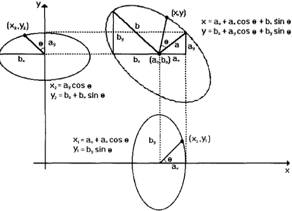
These equations define the image of a continuous mapping for the interval (0, 2n] onto a curve in the plane. Each point corresponds to the locus of end points of the differentiable vector-valued function z(0). The sign ofb x is chosen arbitrarily when the signs of the rotation matrix are defined. These signs imply that three of the axis parameters (ax, ay, bx, by) must be of opposite sign to the fourth. The geometric interpreta- tion of the parameters can be seen in Fig. 1. With this representation the coordinates of a rotated ellipse are defined by two ellipses without rotation whose centres lie on the x and y axes, respectively. These ellipses are used to related the parameter 0 to two of the axis parameters. Then the results are extended for a general ellipse description by considering the rotation. F o r simplicity, xp(0) and yp(0) will now be denoted as x and y.

Parameter space decomposition 371

Y,

• . bo + a , c o s e + bs sin e

Y2 = bo + b. sin e , " % ~ i j

xl= ao÷ a . c o s o Y, = by sin e

(x,,y,)

Fig. 1. Definition of ellipse parameters.

maining parameter can be computed considering the orthogonality of the axes:

a" b = axb x + ayby = 0. (6)

The orientation, p, and the axis (a, b) of the natural parameterization of an ellipse are related to the polar parameterization by:

tan(p) = a~,, a x

a = x / - ~ + a 2, b = ~ + b ~ . (7)

3. FIRST DIRECTIONAL DERIVATIVE ON CIRCLES AND ELLIPSES

The two-plane HT for circles decomposes the three- dimensional parameter space, by using edge tangent normal direction, to map points into two accumulator planes. In this section we consider the direct extension of the technique to ellipses by using the parametric polar form defined by equation (6).

First we show how it is possible to obtain a represen- tation of a circle from directional derivatives of polar functions by involving the edge tangent normal direc- tion computed from an image. Then, this result is

directly generalized for ellipses, establishing the need for using the second directional derivative to obtain a useable decomposition of the parameter space. In section four the two expressions of the two plane HT for ellipses are presented.

3.1. Two-plane H T for circles

Edge direction information computed from an im- age will be denoted by q~'x and ~b'y, which correspond to the tangent and cotangent of the angle inclination (qS) of the tangent line to the ellipse with the positive x axis, as illustrated in Fig. 2.

dy dx

4"x = ~ = tan(4~), ~b' r = ~yy = cot(4~). (8)

The relationship between the polar representation of a circle in equation (1) and the normal gradient computed from an image can be found through the chain rule of differentiation. The tangent of the angle of the position vector function z' is:

dy y' dO dy

= - cot(0), (9)

x' dx dx dO

y'

Z

C y

p o s i t i o n vector funcUon and derivatives Z = x Ux+y U~ U× = (0,1) Z'= x'Ux+y' Us 4 = (1.0)

x

derivatives computed locally d~

tan ~ = ~ - d×

c o t ~ = ~ -

Fig. 2. G e o m e t r y of the derivatives of an ellipse.

thus

~b~, = tan(q~) = - c o t ( 0 ) , ~b'y = cot(~b) = - t a n ( 0 ) . (10)

In order to obtain an expression for x and y as a function of ~b, we substitute the value of cos(0) in equation (1) which defines x via the expression for x'.

Hence:

N/ x'2 (11)

r = (x - ao) 1 + (x - ao) - - - ~ "

Since

then

X'2 r 2 sin2(0)

(x - ao) 2 = ~5 cos2(0) - tan2(0) = ~b~, (12)

r = ( x - ao)`/1 + q~z. (13)

Analogously, by using the definition of y and y' in equation (1), we obtain

r = (y - bo)x~. 1 + q~,2. (14)

Then, based on equations (13) and (14) it is possible to reduce the 3D accumultor required for circle extrac- tion to two 2D accumulators defined by the (ao, r) and (bo, r) parameter spaces.

By considering the trigonometric identities csc2(~b)-- 1 + cot2(~b) and sec2(~b) = 1 + tan2($) in equations (13) and (14), the representation of a circle involving edge.tangent information is perpendicular to its polar representation. That is:

x = a o + r s i n ( d p ) , y=bo+rCos(d~). (15)

This result is clear since equation (10) implies that the angles 4~ and 0 are related by $ = 0 + n/2. Conse- quently, cos(0) = cos(4~ + n/2) = sin(q~) and sin 0 = sin(~b + n/2) = cos(q~).

Alternatively, equations (13) and (14) can be com- bined with equation (15) in order to define a circle extraction process d e c o m p o s e d into two sequential stages, with the accumulators (ao, bo) and (r). The m a p p i n g for the circle centre is then defined by:

y - bo ,/1 + ~'}

x -- a o ~ = q~'y' (16)

and after a o and b o are computed, equations (13) or (14) can be used to c o m p u t e the radius r.

3.2. Extension of the two-plane H T from circles to ellipses

The two-plane H T presented in the previous section can be directly extended to the polar definiton of an ellipse. First, we shall include the information of the first directional derivative on the unrotated ellipse on the x axis in Fig. 1. Then the rotation parameter is included to obtain the complete definition of an ellipse. The expressions for the ellipse without rotation, centred on the x axis, and its first and second direc-

tional derivatives are:

xl = ao + axCOS(0), Yl = bysin(0),

x'l = - ax sin(0), y~ = by cos(0), (17) x~ = - ax cos(0), y~ = - by sin(0).

Analogously to equations (11) and (14):

ax = (x I - a o ) ` / 1 + tan2(0),

bx = (Y2 - bo)`/1 + cot2(0) • (18)

F o r an ellipse the angle 0 and ~b are related by the value of b / a x. Edge direction information computed from an image for an ellipse without rotation is:

y'_~l = _ b y cot(O) ' x'l ax tan(0)" (19)

x'l ax Y'I by

Then the expressions that include the first direc- tional derivative in the definition of an ellipse are obtained by combining equations (18) and (19),

J x,12b2 ax = (x 1 -- ao) 1 + ,--2--2,

Yl ax

j

2

y l 2 ar (20)

bx = (Y2 - bo) 1 q x~ 2 b2.

If the ellipse is rotated by an angle p the values of

y'l/x'l and y'2/x'2 correspond to the tangent and cotan- gent of the angle (0 - p) (see Appendix A):

-axck'y - 1 , ay C~,x

x ' l _ ay , Y--£= - - a x (21)

Y'I ax q~, x~ l + a y q b "

y

ay a x

Therefore, equations (20) for a rotated ellipse become:

4/ [ax'C",+a,l~b~a2

a x = ( X x - - a o ) 1

+ l_ax----~avck----~y

j

x/

-

aye

bx = (Y2 - bo) 1 + F ay ax~b~'] 2 _{t "~"2"} (22)

Lax + a/kxd bx

A l t h o u g h when including the first derivative in the

definition of a n ellipse we obtain a decomposition of

the parameter space into two four-dimensional accu-

mulators (a o, by, a x, ay) and (b o, b x, a x, ay), this result

does not represent a useable decompositon of the parameter space because the dimensions still imply large c o m p u t a t i o n a l and storage requirements. In or- der to handle this, it is necessary to include more information within the polar definition of an ellipse.

4. TWO PLANE HT FOR ELL1PSES

Parameter space decomposition 373

4.1. Second directional derivative on an ellipse

In order to obtain an expression which involves the two parameters which define the centre of an ellipse, we follow equation (16) which relates the two centre parameters of a circle. In the case of an ellipse defined by equation (5) this relatonship becomes:

y - b o = ay cos(0) + by sin(0) (23) x - a o ax cos(0) + b~ sin(0)"

This expression is not equal to the angle of the first derivative but of the second derivative. Hence the relationship of the parameters of the centre of an ellipse is achieved by including the second directional derivative:

y - b o y"

q~ (24)

x -- a o x"

Notice that this is a general case of equation (16) because for a circle ~b'y = ~b~ (isotropy). It is easy to show that this equation combines the geometrical properties of two ellipse points and their tangents (see Fig. 3), and it has been previously used to estimate ellipse centres.~ 12)

Since the relationship betwen 0 and q~ depends on the value of b i G , the axis parameters cannot be obtained following a substitution as in equation (11). Nevertheless, the orthogonality of the ellipse's axes can be used to eliminate 0. By considering the unrotated ellipse defined in equation (17), we obtain the express- ions which define the tangent of the angles of the first and second derivatives:

bY cot(0), "

y'l _ y__L~ = b~ tan(0). (25)

x 'l a x x '~ a x

These equations can be combined in order to obtain an expression that contains the axis parameters of an ellipse:

y'~ y'~ b~ (26)

x'l x'~ a 2"

We generalize this equation to include the orienta- tion by means of the angles of the directional deriva-

y.

.

/

" ~ T

×

Fig. 3. Geometrical relationship between two points on an ellipse and their tangents.

tives computed on a rotated ellipse (Appendix A):

4"x- a~ ~

ay

ax ax b~ (27)

1 +aYG 1 + aY4,:

a~"

a x a x

Although this expression contains three axis para- meters it only relates the ratio between ellipse axis parameters defined by:

ar (28)

N = br K = - - ,

a x a x

then equation (27) defines an expression for an accu- mulator (N, K) as:

~b' x - K ~ : - K = - N Z " (29)

1 + K G 1 + K4,"

Equations (24) and (29) allow the computation of the

parameters of an ellipse by usng two independent accumulators, (ao, bo) and (K, N). After computing the values for ao, bo, K and N, the remaining parameters of the ellipse which corresponds to the value of one axis, can be used to match the values obtained for (ao, bo) with the values obtained for (K, N). In order to obtain the value of a x from the values of (a o, b o , K , N ) we consider the case of an ellipse without rotation centred in the origin defined by:

x o = a cos (0), Yo = b sin (0). (30)

Due to the orthogonality of the axes we know that

b x = - N a x and by = N G. By considering equation (7) we have:

b = Na. (31)

Solving sin(O) from the equation which defines x o in equation (30) we rewrite Yo as:

Yo = N ~ X2o. (32)

For a general ellipse we know that a = ~ + a 2) with

ay = Ka x, consequently:

/y2+_ x 2 N 2 (33) a x = x/S2(1 + K2)"

Due to the definition of xo and Yo these values in a general ellipse must be obtained by translating to the origin and by rotating by - p degrees. Since tan(p) = a j a x = K, then:

1 K

cos(p) ~ , s i n ( p ) = ~ , (34)

and the values of x o and Yo are defined by:

(x -- ao) (y -- bo)K Xo ~ ~ ,

(x - ao)K (y -- bo)

+ - - (35)

After a x has been computed, the other parameters can be obtained by:

ay = ax tan(K), b r = a~ tan(N). (36)

Then, based on the second directional derivative, it is possible to decompose the parameter space into two independent accumulators which define the centre parameters (ao, bo) and axis parameters ( K , N ) , equations (24) and (29), respectively. A final histogram accumulator [equation (33)] allows computation of the remaining ellipse parameter. The complete definition of the ellipse in parametric or normal form can be obtained following equations (34), (36) and (7).

4.2. Computation o f the first and second directional derivatives f r o m an image

In this section we consider the computation of the angle of the first and second directional derivatives by studying image information. It is important to notice that there is no relationship between the second de- rivative computed from an image and the second directional derivative. It is not possible to compute information about directional derivatives of high or- der from derivatives computed from an image. Here, in order to compute the angle of the second directional derivative, we consider two points on an ellipse. We establish that the ratio between second directional derivatives of parametric polar functions is completely defined by two points on the ellipse and their deriva- tives computed from an image. The basic idea is that for each pair of border points on the ellipse (P1, P2), there exists.another point P for which it is possible to compute the values of the angle of the first and second derivatives. Therefore, equations (24), (29) and (33) can be used to compute the ellipse parameters.

The tangent lines of two arbitrary ellipse points P~ and P2 are defined by (see Fig. 3):

YI = c~'x~xl + bl, Y2 = (9'x2x2 + b2. (37)

Based on the polar point T, given by the intersection of these lines:

Y2 - ~ , : x 2 - Yl + 4~,~xl t

X T = C x l - - ( D ' X 2

yl¢'x~ - y24~x, + 4;~4;~:(x2 - x O

Yr - ~b'~ - q~'x~ , (38)

and the middle point M, we derive the relationship between the points P1, P2 and P. Since this relation- ship does not depend on the rotation and position (translation) of an ellipse, it can be obtained by con- sidering an ellipse without rotation centred on the origin. In this case the points are defined by:

x a = axCOS(Oa) , x2 = a x C O S ( 0 2 ) , X e = a~cos(Oe) , Yl = by sin(0 0, Y2 = bysin(02), Ye = by sin(0e).

(39)

In order to obtain the value of 0 e, we compute the

intersection of the line MT with the ellipse. That is:

tan(0r) = a:, YM. (40)

by x M

By substitution of the values of Y u and x u , defined as the average of the coordinates of the points P~ and Pz.

tan(0e ) _ a x by sin(0 0 + by sin(02)

br axCOS(O1 ) + a x C O S ( 0 2 ) , (41) and

tan(Or) =tan(½(O 1 + 02)), (42)

consequently:

0 e = I(01 + 02). (43)

An expression for the angle of the first directional derivative in P is obtained by substitution of this expression in (25):

y-- = _ by cot(Oe ) = _ by cot(½(O1 _ 02))

X r a x a x

by cos(k(01 + 02))sin(½(O~ - 02)) a x sin(l(01 - 02) ) sin(½(O2 - 01) )

= by ( sin(02)- sin(0 0

a:, \ cos (02) - cos(01) J ' (44)

then the angle is:

Y' Y2--Yl

- - - . ( 4 5 )

X r X 2 - - X 1

Similarly, an expression for the angle of the second directional derivative is:

y~; _ by tan(0v), (46)

X~, a x and considering equation (40):

Y~; YM

- = tan(7). (47)

X p X M

where ~, is the angle from the ellipse centre to the point P.

Notice that this result is true for an ellipse centred on the origin. If the centre of the ellipse is (a o, bo) then:

YM - bo

tan(y) . (48)

X M - - a 0

Since we want to use this equation in an expression that relates the values of the axes and not the centre we prefer to write this angle in terms of the points M and T (see Fig. 4). Thus,

tt

Ye Y T - - Y M (49)

X p X T - - X M

By substitution of the values of M and T we find a simplified version of this equation:

y~, A C + 2BD

Parameter space decomposition 375

(a)

('o)

(c)

(d)

(e)

i a x

(n

where

A = y ~ - y 2 , C = Cx, + ¢~, B = x z - x I, D = ¢ ' , o ¢ ~ , r

Equations (45) and (50) can be used to compute the directional information required in the parameter space decomposition presented in Section 4.1.

5. I M P L E M E N T A T I O N A N D RESULTS

In this section we present the implementation and results of an ellipse detection algorithm following the space decomposition achieved by using directional information. It is important to notice that the expres- sions previously presented only define a voting rule for mapping the image space into a parameter space. Our implementation includes considerations which pre- vent bias in the computed values, and which reduce noise in the accumulators caused by pairing points from different objects in an image.

In order to implement equations (24) and (29) it is necessary to define the size and resolution of the accumulators. The accumulator (ao, bo) and the last histogram (ax) are congruent to the image space, there- fore, if we expect that the ellipse is completely con- tained in the image, they are bounded by the image dimension and their maximum resolution is one pixel. As the (N,K) accumulator relates two tangents, it involves an infinite range of values and therefore it does not suit the HT approach directly.

In order to handle the range of the values of K, N we bound the accumulator by storing the angles defined by the values of atan(K) and atan(N). This new accu- mulator has a size of n and its resolution can be related to the image dimensions by considering the accuracy of angles allowed in the discrete irfiplementation. Here we define the range for atan(k) and atan(N) as [--~t/2, ~/2) and [0, 7t) respectively. With this definition K lies between - 1 to 1, and the value of ay is computed as a fraction of the value of a x. This is convenient because small errors in the value obtained for a~, do not change the ellipse's shape significantly.

The main steps in the implementation are:

(1) Application of an edge detector to obtain gradi- ent magnitude and direction.

(2) For pairs of edge points detected

Compute the angle of directional derivatives by using equations (45) and (50). Increment cells in the parameters spaces (a o,bo) and (K,N) according to equations (24) and (29). The cells increased are those defined by the voting curves obtained varying the values of a o and N.

(3) Detect and store local maxima for each accumu- lator array.

(4) For each stored value of(ao, bo) select the stored value (K, N) which produces the maximum value of a x computed by usng equations (33) and (35).

(5) For each ellipse detected [each pair (ao, bo), (K, N)] compute the value of the axis length using equations (36).

This algorithm is theoretically exact and in the case of edge direction obtained by means of a mathematical expression for an ellipse, it produces a perfect peak in the accumulators. This is therefore equivalent to the result obtained by using a conventional HT. Neverthe- less, for digital images, numerical imprecision and noise can cause distortion within the accumulators in complex images. In order to ameliorate this, we reduce the possible pairs of points in the algorithm by two procedures. First, in order to compute an accurate numerical value of the angle of directional deri~,atives we must avoid pairs which define the points M and T which are too close, as well as pairs of points whose tangent differs by a small amount. Second, in order to accumu- late true ellipse evidence, we must ensure that each edge point in a pair defines the same geometric feature. The first requirement is achieved imposing a filter step to verify that pairs of points used in the voting step (2) define a distance between the points M and T to be within a certain range. This range can be determined according to the image resolution. The second con- sideration is more difficult to realize and can be based on complex analysis of an image. Here we use two simple intuitive ideas based on distance and concavity. We impose a distance restriction between paired points since closer points are more likely to belong to the same primitive. The definition of this distance is based on a trade-off between a small value which gives a high probability that each point in a selected pair belongs to the same object and a large value which allows the computation of accurate numerical quanti- ties in the algorithm.

In addition to distance, we consider that a point on an ellipse represents an extremum, consequently, pairs of points belonging to the same ellipse must be in- cluded in the regions defined according to the concav- ity of the curve. We avoid complex computations of curvature and simply consider the limit of the region of concavity in each point by the line whose slope is defined by the gradient direction computed by the edge detector of step (1). In order to estimate whether the region of concavity is either up or down the line defined, we observe the sign of the line equation when points in a small window are evaluated.

Once the appropriate pairs for the implementation algorithm have been defined, it is necessary to search for pairs of points in order to accumulate evidence. As a pair of points defines another point on an ellipse, in order to accumulate complete evidence it would be enough to carry out step (2) as many times as the number of points on an image. Nevertheless, image noise and imprecision in the computed values make it necessary to increase the number of points per edge to be accumulated.

Parameter space decomposition 377

f - ' . , , % - , ,.-.

~.~ . "-~'.~k:-

.. ,~...

,ql~

F

d

fr.,,-, ;%

...

"~--~-

/ ~ ~.;.., .--"

i

)/

"

/ i k ,

,,..,_~ .... , ~...; ., : . ,

. , / ' , , r . , . ' r - ,,', " - " : : " " L .

• ~.~,. ,',, \ ' - -

H-'u ' ,' ' I x !r"--x J " ' ~

'.',

\,tl

) /

/-_,_..

(a)

(b)

(c)

(d)

(e)

(t)

t ~'l.c," ,-~,

,

,/ J

'.t

,~/I" ~,,.

-T.~

':I~'

'"

t - . . L , - " - " - " ' - ~ < _ - • .-

,i<.

,,4' $,,

(a)

~)

(c)

(d)

(e)

( 0

(aO

~lx

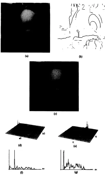
Fig. 6. Detection example of two similar ellipses. (a) Raw image; (b) result of the edge detector operator; (c) result ellipse superimposed; (d) centre accumulator; (e) axis ratio accumulator; (f) a x histogram for the big

Parameter space decomposition 379

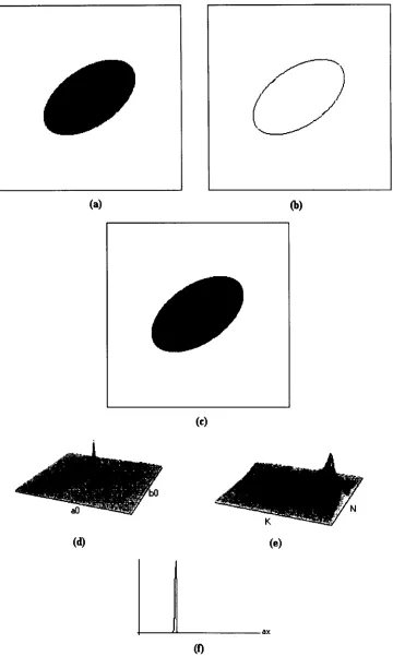
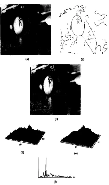
over several accumulator cells, hence the resulting peak becomes wider. Figure 5 shows the results of applying the algorithm to a 256 x 256 x 8 bit image. Figure 5(a) shows the raw image and Fig. 5(b) shows the result of applying the Canny operator. Figure 5(c) displays the detected ellipse superimposed in black. Figures 5(d), 5(e) and 5(f) show the resulting accumula- tors. In the implementation we search for 35 points per edge in order to accumulate significant ellipse evi- dence. Pairs of points are only considered in the voting step if: (1) they are at a distance of less than 130 pixels, (2) they define points M and T between 15 and 400 pixels far apart and (3) they include each other in the region of concavity of the curve that each one defines. The (a o, bo) accumulator has a 256 x 256 resolution, the (atan(K), atan(N)) accumulator has a 100 x 100 resolution and the a x histogram contains 150 pixels.

The important problem for complex images in the previous implementation is that peaks tend to have a wide base, which can lead to errors in the estimation of peak positions for ellipses whose parameters are similar. When the parameters of two ellipses are close, their peaks merge forming a wide plateau with two very small peaks which can be easily confused in the presence of noise.

In order to increase robustness it is necessary to compute more accurate information (e.g. by using an image of higher resolution to compute the edge direc- tion). Here we exploit the coherence of information that exists within small windows in the image in a simple multiple window parameter transform. (13) We consider that because closer points have a high prob- ability of belonging to the same geometric feature (object), they must contribute to the accumulation of the same parameters. Hence we increase accuracy if we only use, as evidence, values supported by sets of points in a small region in an image. Then for a window in the image we carry out a local accumulation step. The maxima in the local accumulator is used to in- crease the global accumulator. As only a large window can produce an accurate value of the parameters of an ellipse, when small windows are considered it is con- venient to include additional values close to the maxi- ma in order to accumulate evidence for the global accumulator.

We apply this double step HT to the image shown in Fig. 6(a). This image contains two ellipses with similar centre and axis ratios K and N. In order to accumulate strong evidence we consider a small window for each edge point by randomly searching for 15 close points within a distance of 15 pixels. After a local accumulator is computed, the cells in the local accumulator which are within 25% of the maximum value are added to the global accumulator. The use of a percentage allows sharp local peaks which represent high local evidence to vote strongly for a few values, while small wide peaks which represent local uncertainty vote weakly for many possible values. Figures 6(b) and 6(c) show the data used for the algorithm and the resulting ellipses. Figures 6(d) and 6(e) show how the double

voting process produces two sharp peaks for para- meters with similar values. Figures 6(f) and 6(g) show the histogram for the large and the small ellipses respectively.

6. CONCLUSIONS

The inclusion of edge direction information in an analytic description of an ellipse can be used to define a mapping which decomposes the parameter space required for the HT into two independent sub-spaces. As parameter space decomposition constitutes an ef- fective approach to reduce both the time and space requirements in the HT, the use of edge direction provides a feasible alternative for extracting ellipses.

The mapping defined here exploits regularities on continuity information, therefore, clutter edges influ- ence the results less than when only edge position data is considered. The robustness of the presented tech- nique depends on the accuracy of computation of edge data, this highlights the importance of the identifica- tion of image regularities for extracting primitive el- ements from an image. In this sense we recognize the problem of primitive extraction as the process of form- ing geometrical models based on the computation of image structures, which can contribute incrementally to the evidence of the shape.

Information on complex image structure available within an image can be used to reduce the number of possible interpretations of primitives in an image. This information defines constraints in the spatial structure in the image, for example by means of point configur- ations defined geometrically by relative positions. In this paper we addressed the problem of including information computed locally in order to reduce poss- ible image interpretations on ellipse extraction.

We conclude that the reduction of possible interpre- tations requires a sophisticated analysis of image data, and that besides considering constraints in geometric features defined by the primitives in an image, it is important to study how models based on complex information available from an image (e.g. edge direc- tion) can accumulate evidence of data organization.

Acknowledgements--The authors would like to express their thanks to C. Davies for implementation of the Canny edge detector operator. A.S. Aguado and M.E. Montiel are grateful to the CONACyT (Consejo Nacional de Ciencia y Tec- nologia, M~xico) and to the DGAPA (Direccion General de Asuntos del Personal Acad6mico) from the UNAM (Univer- sidad Nacional Aut6noma de M6xico) for their financial support.

REFERENCES

1. R. D. Duda and P. E. Hart, Use of the Hough transform to detect lines and curves in pictures, Commun. ACM

15(1), 11-15 (1972).

2. J. Illingworth and J. Kittler, A Survey of the Hough transform, Comput. Vis. Graphics Image Processing 44(1),

87-116 (1988).

3. V. F. Leavers, Which Hough transform? CVGIP: Image Understanding 58(2), 250-264 (1993).

4. J. Illingworth and J. Kittler, The adaptive Hough trans- form, I E E E Trans. Pattern Anal Mach. lntell. 9(5), 690- 697 (1987).

5. R.S. Conker, A dual-plane variation of the Hough trans- form for detecting non-concentric circles of different

radii, Comput. Vis. Graphics Image Process. 43(1), 115-

132 (1988).

6. S. Tsuji and F. Matsumoto, Detection of ellipses by a modified Hough transform, I E E E Trans. Comput. 27(8), 777-781 (1978).

7. H. K. Muammar and M. Nixon, Tristage Hough Trans-

form for multiple ellipse extraction, I E E Proc. E 138(1),

27-35 (1991).

8. D. Pao, H. F. Li and R. Jayakumar, A decomposable

parameter space for the detection of ellipses, Pattern

Recognition Lett. 14(12), 951-958 (1993).

9. R.K.K. Yip, P. K. S. Tam and D. N. K. Leung, Modifica- tion of Hough transform for circles and ellipses detection

using a 2-dimensional array, Pattern Recognition 25(9),

1007-1022 (1992).

10. J. H. Yoo and I. K. Sethi, An ellipse detection method

from the polar and pole definition of conics, Pattern

Recognition 26(2), 307-315 (1993).

11. W. Wu and M. J. Wang, Elliptical object detection by

using its geometrical properties, Pattern Recognition

26(10), 1499-1509 (1993).

12. H. K. Yuen, J. Illingworth and J. Kittler, Detecting partially occluded ellipses using the Hough transform, Image l/is. Comput. 7(1), 31-37 (1989).

13. A. Califano and R. M. Bolle, The multiple window par-

ameter transform, 1EEE Trans. Pattern Anal. Math.

lntell. 14(12), 1157-1170 (1992).

A P P E N D I X A

In this appendix we show the relationship between the tangent of a rotated ellipse and an ellipse centred on the x-axis (see Fig. 1). We first consider the angle measured in a rotated ellipse which according to equations (1) and (8) is:

x' - a x sin(0) + b xcos(0) cot(qS) = --

y' - a y sin(O) + bycos(O)"

Solving for tan(0):

tan(O)

b x

- - - c o t ( q s ) by b r

ax 1 _ aycot(~b)

ax

Since:

then:

x' 1 ax ~-~1= - ~ tan(0),

a ~ c o t ( q s ) - i

x__~]= ay cot(qs-p).

y~ ax cot(S)

ay

Similarly, for an ellipse centred on the y axis:

and

y' - ay sin(O) + by cos(O)

tan(q5) = -- =

x' - a xsin(O)+bxcos(O)'

Y~ bxcot(0) '

x~ ay

then:

consequently:

a~-tan(qs) COt(0)= ax ax

by 1 + a r t a n ( ~ ) '

ax

ar tan(S)

y~ ax

a

x~ 1 +--rtan(q5)

ax

t a n ( 0 - p ) .

(A7)

(A8)

SUMMARY

The Hough transform (HT) is an established technique for extracting geometric primitives represented by parametric curves. The technique defines a mapping between an image space and a parameter space which is used to accumulate evidence of primitives in an image. The main drawback of the technique is that it requires an n-dimensional parameter space for a curve with n parameters. In order to overcome the excessive requirements, in both time and memory for ellipse extraction, current techniques decompose the parameter space into several sub-spaces of reduced dimensions. The decomposition is achieved by using geometric properties of an ellipse. These properties involve geometrical constraints between edge points on an image. These constraints include distance and angular relationships which define relative posi- tions between a set of edge points. Hence, the parameters.of an ellipse are computed after labelling the points which satisfy the constraints, in a computationally intensive approach. The aim of this paper is to show how directional information can be used to derive a mapping which decomposes the parameter space required for the application of the HT. In order to

(A1) obtain explicit expressions which constitute simplified map-

pings between the image space and the parameter space, we use the parametric polar representation to combine geo- metric data with directional information. Based on the parametric polar representation we extend the use of directional information from circle to ellipse detection. We

(A2) show that, due to the ellipse anisotropy, it is necessary to

involve the information of the second directional derivative in order to obtain a useful decomposition of the parameter space.

The use of the second directional derivative allows the definition of a mapping which decomposes the five

(A3) dimensional parameter space required for ellipse ex-

traction into two independent sub-spaces, each of which relate two ellipse parameters. A final histogram accumu- lator is used to obtain the remaining parameter. The major difference between previous approaches and our approach is the consideration that two ellipse points define the ratio

(A4) between directional derivatives, of first and second order, of

the parametric polar function of another point. We show how the directional information included in the defined mapping can be computed by considering two points and their gradient direction. The most important result of this paper is that the use of gradient information for parametric decomposition avoids the constraints which

(A5) define relative positions between a set of points required

by other approaches. We present an implementation includ- ing considerations which prevent bias in the numerical values computed from an image and which reduce noise in

(A6) the accumulators caused by pairing points from different

Parameter space decomposition 381

About the Author--ALBERTO AGUADO completed his B.Sc. degree in computer science in 1989 from La Salle University, M6xico. In 1992 he received an MSc. (Hons) in computer science from the Universidad Nacional Aut6noma de M6xico and an M.Sc. (Hons) in planning and systems with specialization in operations research from La Salle University. In 1993 he started a Ph.D. at the University of Southampton in the Image, Speech and Intelligent Systems (ISIS) research group in the Department of Electronics and Computer Science.

About the Author--M. EUGENIA MONTIEL completed her B.Sc. degree in computer science in 1989 from La Salle University, M~xico. In 1992 she received an M.Sc. (Hons) in computer science from Universidad Nacional Aut6noma de M6xico and an M.Sc. (Hons) in planning and systems with Specialization in operations research from La Salle University. In 1993 she started a Ph.D. at the University of Southampton in the Concurrent Computation research group in the Department of Electronics and Computer Science.

About the A u t h o r - - M A R K NIXON is a lecturer in electronics in computer science and is a member of the