Optimising strategy selection for the management of railway assets

Optimising strategy selection for the management of

railway assets

C. Fecarotti and J. Andrews

Resilience Engineering Research Group, The University of Nottingham, United Kingdom.

ABSTRACT

In the railway industry a main concern is how to manage efficiently and effectively the railway assets under budget constraints. Optimal asset management involves decision making and selection of the best inspection, maintenance and renewal interventions for each asset along the network. This paper presents an optimisation method for supporting the decision making process. The method is based on a two-level approach. At a lower level, asset models combining degradation and intervention processes are used in order to evaluate the effects of different intervention strategies on the evolution of the asset state over time. On a system-level, a Knapsack-type optimisation model is developed to selects the optimal combination of intervention strategies to apply to all assets in the network in order to deliver the required level of performance while minimising the whole lifecycle costs.

1. BACKGROUND

The management of railway assets is a complex process combining periodic inspection, routine and emergency maintenance, enhancement and renewal activities. Decisions need to be made on when and how these activities must be carried out in order to ensure that a given level of service and safety is achieved while satisfying budget constraints. The railway asset management strategy selected will have a direct effect on the reliability of the railway service as well as passengers’ safety. The railway system consists of several assets which are all very diverse in nature, and all contribute to the overall system performance. Each asset is affected by specific deterioration and failure processes and requires appropriate interventions to maintain the asset to an acceptable state. It is fundamental to investigate the effects of different intervention strategies on the evolution of the asset conditions over time in order to inform the decisions on strategy selection and resources allocation. Optimal asset management involves decision making and selection of the best intervention strategy for each asset along the network. When a network perspective is adopted, asset and route criticality need to be considered. Furthermore, dependencies among different assets and different sections of the network arise, due for example to resource availability. This implies that intervention strategies that are optimal when an asset is considered individually, might not be optimal when decisions are made at a network level.

This paper presents a methodology for the optimisation of intervention strategies for the railway infrastructure system. The methodology consists of a two level approach. First, asset models combining degradation/failure and intervention processes are used for individual asset type in order to evaluate the effects of different intervention strategies on the evolution of the asset state over time. Then a network-level optimisation model is developed in order to support the selection of the best intervention strategy to apply to each asset, subject to budget availability and performance constraints. The network-level optimisation model is formulated as a knapsack problem with multiple constraints which is a stylised model in mathematical programming (1). The model is bounded to select one option for each individual asset along a section of the railway network to maximise the overall performance. Budget availability and performance requirements such as lines availability are formulated as model constraints. The model also takes into account as route criticality by attributing different thresholds to the availability of each route. It has the advantage to easily allow for the evaluation of a variety of different scenarios by changing the model parameters such as the available budget or the threshold levels set for the asset availability. The methodology is demonstrated here for selecting the best intervention strategy to apply to the track asset for a section of the railway network. Future work will expand the model in order to consider different asset types.

optimisation approach to optimise inspection and maintenance procedures with respect to both economical and safety-related aspects.

2. METHODOLOGY

The methodology proposed in this paper consists of a two level approach. First, asset models combining degradation/failure and intervention processes are used for individual asset type in order to evaluate the effects of different intervention strategies on the evolution of the asset state over time. Then a network-level optimisation model is developed in order to support the selection of the best intervention strategy to apply to each asset, subject to budget availability and performance constraints. The asset models are used to inform the network level optimisation model by providing indication of the effects of a given set of intervention strategies on the conditions and performance of the asset. In the next section a track asset model is developed using the Petri net method. Then, a brief introduction is given to the Knapsack problem from which the network-level optimisation model is derived.

2.1. Track asset model

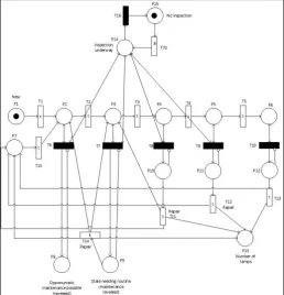
The passage of traffic along the railway network leads to track geometry degradation which has a direct effect on safety and on the reliability of the service. Track geometry inspection is performed periodically by running Track Recording Vehicles along the network to evaluate the state of the track. The vehicle measures the location of the rails and provides the variations of the rails vertical and horizontal position, gauge, twist and cyclic top over 1/8th _{mile section. Based on the output of the inspection process, remedial works are scheduled} if necessary. If the state of the track is revealed to be above a safety threshold, than a speed restriction or even a line closure can be issued while an emergency repair is scheduled and performed. The time required to perform the intervention depends on the severity of the degraded state. The short-wave vertical profile of the two rails is usually considered as the most significant measurement when planning the maintenance activities. In particular this vertical profile is given by the mean of the two rails height standard deviation when considering 35 m wave-length. Ballast degradation is the main cause of variation in vertical rail geometry. Tamping machines or sometimes manual adjustment, are used to improve geometry conditions. However, while improving track geometry conditions, tamping also damage the ballast, causing the track geometry degradation rate to increase over time with the number of tamping performed (5).

In this section an integrated track geometry and maintenance model is presented. The model represents a 1/8th mile section of track and describes the phased degradation process of the track geometry along with the inspection, routine and emergency maintenance processes. Multiple instances of this model are then created to generate a track section model of the required length. The modelling methodology adopted is the Stochastic Petri net (8). Petri nets are a formalism for modelling complex distributed systems characterised by concurrency and dependency, synchronization and resource sharing. Petri nets provide a valuable mathematical and graphical description of the system behaviour. A Petri net is a directed, weighted bi-partite graph where nodes are places and transitions connected by arcs (7, 8). Places may represent physical resources, conditions or the state of a component. Tokens are held in places and the number of tokens in each place, referred to as marking of the Petri net, represents the state of the system at a given time. The flow of tokens through the network represents the dynamic of the system and is governed by transitions. Transitions represent events that make the status of the system change. Arcs only connect places with transitions (input arcs) and vice versa (output arcs). A particular type of arc called inhibitor can be used to stop the firing of a transition under certain circumstances. Arcs are characterised by a multiplicity. The marking of the net along with the multiplicity of the arcs determine the enabling conditions for each transition. Petri nets in which a firing time is associated to transitions are called Timed Petri net. Furthermore, this firing time can be either deterministic or stochastic. In the latter case, the firing time of the stochastic transitions is sampled from the appropriate stochastic distribution. Firing of transitions is ruled as follow:

 The transition must be enabled, namely the number of tokens contained in the input places must be at least equal to the multiplicity of the associated input arcs, and the number of tokens in the places connected by inhibitor arcs must be lower than the arcs multiplicity.

 Once the transition is enabled, the transition will fire after a period of time t whose value depends on the type of transition. Deterministic transitions have an associated fixed firing time which is 0 for immediate transitions. For stochastic transitions the firing time is sampled from a probabilistic distribution.

 When the firing time is reached and the transition fires, a number of tokens is removed from the input places, which is equal to the associated arc multiplicity. Analogously, a multiplicity of tokens is added to the output places.

In a PN places are represented by circles, transitions by rectangles and tokens by small black dots contained into places.

inspection is underway, while P15 is marked when no inspection is performed. Transition T17 will fire at fixed intervals depending on the inspection frequency θ, indicating that the inspection process has started. Transition T16 represents the end of the inspection. When P14 is marked, it will enable transitions T7 to T11 which will simply reveal the current state of the track. The revealed states are represented by places P8 to P12. Maintenance, both routine and emergency, is triggered by a revealed state requiring intervention. Transitions T11 to T13 represent emergency repairs while transition T14 represents the routine maintenance. The time to schedule and perform maintenance and repair processes is normally distributed and therefore transitions T11 to T14 are stochastic transitions with firing time sampled from a normal distribution. The model also account for the fact that the effectiveness of the maintenance process can vary. When maintenance has been carried out, and therefore one of transitions T11 to T13 has fired, the state of the track can be brought back to either a good state (place P7 will be marked) or worst. However, since in real situation it is very rare that the state of the track following maintenance is such to require a speed restriction or a line closure, the possible state following maintenance are only the ones indicated by places P2, P3, P4 and P7.

Figure 1 Track geometry degradation and maintenance model.

In order to form a track section model, multiple instances of the track degradation and maintenance model are generated and linked together according to the dependencies between adjacent sections. Two types of dependencies have been considered here in order to build the track section model: the inspection process and the opportunistic maintenance. An example of track section model is shown in Figure 2.

When the state requiring routine maintenance is revealed in one of the track geometry degradation and maintenance modules (1/8 mile section), the state of the adjacent modules within a given distance is checked. If any of the adjacent modules is found to be in a state where opportunistic maintenance is suitable, then an intervention for routine maintenance will be performed on such modules too. The chain of places and transitions at the bottom of Figure 2 represents the process of sequentially checking the state of the modules adjacent to the one currently needing routine maintenance. Due to the stochasticity of the deterioration and intervention processes, Monte Carlo simulation is used to analyse the track section PN model. Several information such as the number of tamping interventions or the number of imposed speed restrictions can be recorded during the simulations. In order to provide the input necessary to the network level optimisation problem presented in the next section, the following output are required from the track asset model: probability of line closure, number of speed restriction, number of interventions (tamping) per lifetime.

2.2. Network level optimisation: The optimal railway asset management problem

2.2.1. The Knapsack problem

The Binary Knapsack Problem is a mathematical optimisation problem belonging to the class of Binary Integer Programming (1). In its canonical form it is formulated as follow.

Given a set of items N={1,2,...n} each characterised by a value vi and a volume wi, and a knapsack with volume b, the objective is to select a subset of the items in order to maximise the value of the knapsack without exceeding its volume.

max ∑ 𝑣𝑖∙ 𝑥𝑖 𝑖∈𝑁

[1]

𝑠. 𝑡.

[1.1] ∑ 𝑤𝑖∙ 𝑥𝑖 ≤ 𝑏 𝑖∈𝑁

[1.2] 𝑥𝑖∈ {0,1} , 𝑥𝑖{1 𝑖𝑓 𝑖𝑡𝑒𝑚 𝑖 𝑖𝑠 𝑠𝑒𝑙𝑒𝑐𝑡𝑒𝑑_{0 𝑜𝑡ℎ𝑒𝑟𝑤𝑖𝑠𝑒} .

To each item 𝑖 is associated a decisional variable 𝑥𝑖 which will take value 1 if the item is selected and put in the knapsack, 0 otherwise. The objective function ∑_𝑖∈𝑁𝑣_𝑖∙ 𝑥_𝑖 represents the total value of the knapsack which has to be maximised. Constraint 1.1 indicates that the choice of items have to be such that the overall volume of the knapsack b is not exceeded. The second constraint indicates that the decisional variables are binary; this means that an item can be either put entirely in the knapsack or not chosen at all. In this classical form the knapsack is a linear integer binary model because the decisional variables are all binary and both the objective function and the constraints are linear functions. Standard solution algorithms for mixed-integer programming problems can be used to solve the knapsack problem, such as the branch and bound method or the interior point methods. The description of these solution algorithms is out of the scope of this paper and therefore the reader is referred to (1) for further reading.

In real applications, the decisional variables may represent decisions to be taken. If the problem to solve, for example, is selecting one or more investment strategies among a set of available ones, then a decisional variable associated to each of the available strategies will indicate whether the strategy is selected or not. According to the specific decisional problem to be addressed, the binary knapsack problem can be customised by including additional constraints and by further specifying the objective function based on the specific problem. Furthermore, both the objective functions and the constraints can take a nonlinear form which will simply require solving either a linear approximations of the original problem or applying more sophisticated solution algorithms.

In the next section, the decisional problem of selecting the best intervention strategies to apply to the assets on a section of the railway network is formulated as a Knapsack-type problem.

2.2.2. The knapsack formulation for railway track asset management

{𝑒𝑖} 𝑤𝑖𝑡ℎ 𝑖 = 1,2, . . , 𝐼. The set of available strategies is 𝑆 = {𝑠𝑗} 𝑤𝑖𝑡ℎ 𝑗 = 1,2, . . , 𝐽. Trains run through the network along a number of railway lines denoted as 𝑙𝑘. The set of railway lines is 𝐿 = {𝑙𝑘} 𝑤𝑖𝑡ℎ 𝑘 = 1,2, … , 𝐾 where each line 𝑙𝑘 consists of an ordered sequence of links 𝑒𝑖. A strategy must be selected for each link in the network. Therefore we define the vector of decisional variables 𝑋 with components 𝑥𝑖𝑗 such that 𝑥𝑖𝑗= 1 if strategy 𝑗 is applied to link 𝑖, 𝑥𝑖𝑗= 0 otherwise. The parameters of the model are:

 𝑛_𝑖𝑗𝑆𝑅 _{the number of speed restriction imposed on link 𝑖 following implementation of strategy 𝑗,}  𝑑𝑖𝑗𝑆𝑅 the duration of speed restriction imposed on link 𝑖 following implementation of strategy 𝑗,  𝑎_𝑖𝑗𝐿𝐶 _{the availability of link 𝑖 following implementation of strategy 𝑗; this is given by 1 − 𝑞}

𝑖𝑗𝐿𝐶 where 𝑞𝑖𝑗𝐿𝐶 is the probability of link 𝑖 being closed following implementation of strategy 𝑗,

 𝐴_𝑙𝑘 the threshold on the availability of line 𝑙𝑘,  𝑐𝑖𝑗 the cost of strategy 𝑗 implemented on link 𝑖,  𝑓𝑖 the frequency of trains travelling on link 𝑖,

 𝐶 the available budget.

The problem can be formulated as follow:

min ∑𝑒𝑖∈𝐸∑𝑠𝑗∈𝑆𝑛𝑆𝑅𝑖𝑗 ∙ 𝑑𝑖𝑗𝑆𝑅∙𝑓𝑖∙ 𝑥𝑖𝑗 [2] 𝑠. 𝑡.

[2.1] ∑ 𝑥𝑖𝑗 = 1 ∀ 𝑒𝑖∈ 𝐸 𝑠𝑗∈𝑆

[2.2] ∑ ∑ 𝑐_𝑖𝑗∙ 𝑥_𝑖𝑗 ≤ 𝐶 𝑠𝑗∈𝑆

𝑒𝑖∈𝐸

[2.3] ∏ (∑ 𝑎𝑖𝑗𝐿𝐶⋅ 𝑥𝑖𝑗 𝑠𝑗∈𝑆

) ∀𝑖∕𝑒𝑖∈𝑙𝑘

≥ 𝐴𝑙∗𝑘 ∀ 𝑙𝑘∈ 𝐿

[2.4] 𝑥𝑖𝑗∈ {0,1} , 𝑥𝑖𝑗{1 𝑖𝑓 𝑠𝑡𝑟𝑎𝑡𝑒𝑔𝑦 𝑠_{0 𝑜𝑡ℎ𝑒𝑟𝑤𝑖𝑠𝑒}𝑗 𝑖𝑠 𝑎𝑝𝑝𝑙𝑖𝑒𝑑 𝑡𝑜 𝑠𝑒𝑐𝑡𝑖𝑜𝑛 𝑒𝑖.

The objective function in [2] provides an indication of the impact that the average number and duration of speed restrictions imposed on each link has on the overall train service across the network. The impact of each link is weighted with the train frequency on the link. The aim is therefore to select a track management strategy for each link in order to minimise such impact. This means selecting a value for each binary variable 𝑥𝑖𝑗 such that the objective function in [2] is minimised while satisfying constraints [2.1] to [2.4]. The set of constraints [2.1] indicates that one strategy must be selected for each link. Constraint [2.2] adds a bound on the overall costs according to the available budget. The set of constraints [2.3] put a threshold on the minimum value of availability of each line. Each line can be seen as a series system where each component corresponds to a link. From reliability theory it is well known that a series system will work only if all of its components work. For such system, the probability of success for the system is given by 𝐴𝑠𝑦𝑠= ∏ (𝑎∀𝑖 𝑖) where 𝑎𝑖 is the availability of component 𝑖 (6). Indeed, the left-hand side of constraint [2.3] indicates the probability of line 𝑙𝑘 being available. Finally, constraint [2.4] indicates that each decisional variable is binary and can therefore only take either value 1 or 0.

3. NUMERICAL EXAMPLE

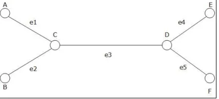
In order to demonstrate the proposed method the optimisation procedure has been applied to the network in Figure 3 for selecting the track intervention strategy to apply to each link. The aim of this section is to give numerical insight into the capabilities of the optimisation model, therefore the values and network used here are only indicative and not representative of a real network.

Figure 3 Graph of the considered railway network.

maintenance and same time to perform emergency repair. The number of speed restriction imposed, the availability of the link and the interventions costs related to each strategy are summarised in Table 1. It is assumed that the track characteristics for each link are the same (homogeneous tracks). Therefore it is possible to assume that, on average, the effect of a specific strategy on each link in terms of number of imposed speed restrictions and link availability will be comparable. For each strategy, it is assumed that costs can vary within a given range to consider that different links may have different accessibility, due for example to the distance from the maintenance depot.

Table 1 Features of intervention strategies.

Strategy no _{of speed restrictions Availability of link Cost of strategy}

S1 4.7 0.9 50-60

S2 3.8 0.95 70-80

S3 2.5 099 85-95

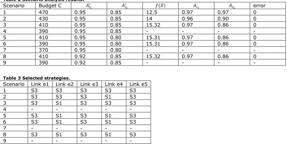
With five sections of track and three possible intervention strategies, the vector of the decisional variables 𝑋 will have fifteen components. The optimisation problem has been solved for different values of the available budget C and threshold availability for line l1 and l2. In particular nine different scenarios have been considered as shown in Table 2 where corresponding value of the objective function 𝑓(𝑋) and lines availability 𝐴𝑙1and 𝐴𝑙2are detailed, along with the error whenever the optimal solution could not be found and an approximate solution has been considered. Table 3 shows the choice of strategies for the different scenarios.

Table 2 Scenario analysis results.

Scenario Budget C 𝐴_𝑙∗_{1 𝐴} 𝑙2

∗ _{𝑓(𝑋) 𝐴}

𝑙1 𝐴𝑙2 error

1 470 0.95 0.85 12.5 0.97 0.97 0

2 430 0.95 0.85 14 0.96 0.90 0

3 410 0.95 0.85 15.32 0.97 0.86 0

4 390 0.95 0.85 - - - -

5 410 0.95 0.80 15.31 0.97 0.86 0

6 390 0.95 0.80 15.31 0.97 0.86 0

7 370 0.95 0.80 - - - -

8 410 0.92 0.85 15.32 0.97 0.86 0

9 390 0.92 0.85 - - - -

Table 3 Selected strategies.

Scenario Link e1 Link e2 Link e3 Link e4 Link e5

1 S3 S3 S3 S3 S3

2 S3 S3 S3 S1 S3

3 S3 S1 S3 S3 S3

4 - - - - -

5 S3 S1 S3 S1 S3

6 S3 S1 S3 S1 S3

7 - - - - -

8 S3 S1 S3 S1 S3

9 - - - - -

In the first scenario (scenario 1), the available budget and the thresholds for lines availability are such that the most expensive strategy (S3) is selected for each link. For decreasing values of the available budget, less expensive strategies are selected in the solution for either link e2 (scenario 2) or e4 (scenario 3) but not for links e1, e3, e5. Indeed links e1, e3, e5 belong to line l1 for which a higher value of minimum availability is requested, while links e2 and e4 belong to line l2 for which a less restrictive threshold for line availability is accepted. This also implies higher values of the objective functions indicating the impact on service due to the number of speed restrictions. By further decreasing the available budget, but keeping the same thresholds for lines availability, no feasible solutions are found (scenario 4). This means that for the available budget, no strategy provides acceptable level of availability for both lines. In scenarios 5 and 6 the same budget as in 2 and 3 respectively is considered, but with less restrictive thresholds for line availability. Strategy S1 is selected for both links e2 and e4 this time, which implies a worst (higher) value of the objective function. By further decreasing the budget (scenario 7) no feasible solution exists. It is worth specifying that, for large instances, optimal solutions may be difficult to find in reasonable computational time. In such cases, it is possible to settle for a “sub-optimal” solution achievable through approximate methods, given that a pre-defined tolerance is respected. A possible way to assess the quality of an approximate solution is based on percentage error. This is defined as the distance between an upper bound provided by the current approximate solution and a lower bound provided by a super-optimal solution. Super-optimal solutions are usually obtained through “relaxation methods” such as the Lagrangian relaxation and Continuous relaxation (1). The Lagrangian relaxation is based on the idea of turning some of the constraints into penalty terms appearing in the objective function and weighted by so called “lagrangian multipliers”. The continuous relaxation method changes the nature of the decision variables from integer to continuous, making the problem easier to solve.

4. CONCLUSIONS

intervention strategies on the evolution of the asset state over time. Then a network-level optimisation model is developed in order to support the selection of the best intervention strategy to apply to each asset along the network, subject to budget availability and performance constraints. The asset models are used to inform the network level optimisation model by providing indication of the effects of a given set of intervention strategies on the conditions and performance of the asset. Numerical examples have been shown to demonstrate the capability of the proposed approach. This approach combines the detailed information on the asset behaviour provided by the PN asset models, with a network optimisation model that allows to consider both functional and economical dependencies arising when a network perspective is adopted. Future work will expand the model in order to consider additional asset types. Furthermore, at this stage, the optimisation model considers only economical (budget constraint) and functional (line availability constraints) aspects. Future developments of the method will have to include safety-related aspects.

AKCNOWLEDGMENT

John Andrews is the Network Rail Professor of Infrastructure Asset Management. He is also Director of Lloyd's Register Foundation (LRF)1 _{Resilience Engineering Research Group at the University of Nottingham. Claudia} Fecarotti is conducting a research project funded by Network Rail. They gratefully acknowledge the support of these organisations.

REFERENCE LIST

1. Martello S. Toth P. (1990). Knapsack Problems: Algorithms and Computer Implementation. John Wiley & Sons, Inc. New York, NY, USA ©1990.

2. Furuya A. Madanat S. (2013) Accounting for network effects in railway asset management. Journal of Transportation Engineering 2013, 139:92-100.

3. Vale, C., Ribeiro, I., and Calçada, R. (2012). "Integer Programming to Optimize Tamping in Railway Tracks as Preventive Maintenance." J. Transp. Eng., 10.1061/(ASCE)TE.1943-5436.0000296, 123-131.

4. Podofillini, L., Zio, E., Vatn, J., (2006). Risk-informed optimisation of railway tracks inspection and maintenance procedures. Reliability Engineering & System Safety 91, 20–35.

5. Audley M. Andrews J. (2013). The effects of tamping on railway track geometry degradation. Proceeding of the Institution of Mechanical Engineers, Part F: J Rail Rapid Transit 2013;227(4):376-391.

6. Andrews J.D. Moss T.R. (2003). Reliability and risk assessment, Second ed. London: Professional Engineering Publishing, 2003.

7. Murata T. (1984). Petri nets: properties, analysis and applications Proc IEEE, 77 (no. 4) (1984), pp. 541–580.

8. David R. Alla H. (2010). Discrete, continuous, and hybrid Petri nets Springer Science & Business Media.