1
Smart Windows – Dynamic Control of Building Energy Performance
12
Kaitlin Allen, Karen Connelly, Peter Rutherford and Yupeng Wu*
3 4
Department of Architecture and Built Environment, Faculty of Engineering, University of Nottingham,
5
University Park, Nottingham, NG7 2RD, UK
6
*Corresponding author: Tel: +44 (0) 115 74 84011; emails: Yupeng.Wu@nottingham.ac.uk, Jackwuyp@googlemail.com
7
Abstract 8
This paper will explore the potential of employing thermotropic (TT) windows as a means of
9
improving overall building energy performance. Capitalising on their ability to dynamically
10
alter solar and visible light transmittance and reflectance based on window temperature,
11
they have the potential to reduce solar heat gains and subsequently reduce cooling loads
12
when the external conditions exceed those required for occupant comfort. Conversely when
13
the external conditions fall short of those required for occupant comfort, they maintain a
14
degree of optical transparency thus promote the potential for passive solar gain. To test
15
their overall effectiveness, thermotropic layers made of varying hydroxypropyl cellulose
16
(HPC) concentrations (2wt.%, 4wt.% and 6wt.%) were firstly synthesised and their optical
17
properties measured. Building performance predictions were subsequently conducted in
18
EnergyPlus for four window inclinations (90°, 60°, 30° and 0° to horizontal) based on a small
19
office test cell situated in the hot summer Mediterranean climate of Palermo, Italy. Results
20
from annual predictions show that both incident solar radiation and outdoor ambient
21
temperature play a significant role in the transmissivity and reflectivity of the glazing unit. If
22
used as a roof light, a 6wt.% HPC-based thermotropic window has a dynamic average Solar
23
Heat Gain Coefficient (SHGC) between 0.44 and 0.56, this lower than that of 0.74 for double
24
glazing. Predictions also show that in the specific case tested, the 6wt.% HPC-based
25
thermotropic window provides an overall annual energy saving of 22% over an equivalent
26
double glazed unit. By maintaining the thermotropic window spectral properties but
27
lowering the associated transition temperature ranges, it was found that the lowest
28
temperature range provided the smallest solar heat gains. Although, this is beneficial in the
29
summer months, in the winter, passive solar heating is restricted. In addition, with lower
30
solar heat gain, there is a possibility that artificial lighting energy demand increases resulting
31
in additional energy consumption.
32
33 34
Keywords: Thermotropic window; smart window; hydroxypropyl cellulose (HPC); building
35
simulation; solar heat gain coefficient.
36 37
1. Introduction 38
Buildings are responsible for 40% of energy consumption within the EU, and consequently
39
contribute to approximately 36% of overall carbon emissions [1]. As has been recognised for
40
example in the UK’s amendments to Approved Document L, the envelope of a building is
41
crucial in terms of energy consumption. Attention therefore needs to be made to the design
42
and specification of the transparent elements that comprise the building’s envelope. Whilst
43
such elements are often considered to be thermally weak, this has to be offset against the
44
benefits to occupant comfort, health, wellbeing and productivity afforded by natural light,
45
views and associated control over natural ventilation. A case can therefore be made to
2
transparent elements whilst maintaining the optical properties that govern daylight
2
availability, view and so on.
3
To maximise the benefits of view and daylight availability, many contemporary
4
commercial and residential buildings employ high levels of glazing. If well designed these
5
can lead to significant heat loss or gains when the external conditions are outside the range
6
normally accepted for occupant comfort and as a consequence may increase the energy
7
demands of the building. Although window technology that aims to stabilise the internal
8
temperature of glazed buildings has improved over recent years, many are static and
9
inflexible, such as low-emissivity (low-e) glazing. ‘Switchable glazing’ however is designed to
10
regulate the amount of transmitted solar and long-wave radiation (300-3000nm) and is
11
therefore far more adaptive in nature. By responding to an applied stimulus; heat
12
(thermochromism), electricity (electrochromism) and light (photochromism), these
13
technologies have demonstrated significant potential to reduce energy consumption in
14
buildings [2].
15
Thermotropic (TT) windows are a type of thermochromic (TC) glazing that features
16
reversible transmission behaviour in response to heat. By employing a manufacturing
17
technique that allows the transition / switching temperature (Ts) to be adapted to suit
18
various climatic forces, it provides a solution that can regulate indoor environmental
19
conditions by controlling solar heat gain and visible light transmittance. If we consider a
20
hydrogel and polymer based example, when the temperature of the thermotropic layer is
21
below a designed Ts, its two main components, hydrogel and polymer, uniformly mix
22
resulting in the layer appearing transparent. Conversely, the layer becomes translucent and
23
diffusely reflecting when Ts is exceeded due to the two components having separated [3, 4].
24
As such, in its translucent state it reduces the amount of solar radiation entering a building
25
during hot periods therefore potentially reducing overall cooling loads. In its transparent
26
state, solar radiation is admitted to the building thus contributing to external heat gains.
27
Whilst the exact positioning of thermotropic glazing is in the hands of those responsible for
28
the building’s design, its use is more suited to areas where an obstructed view is not
29
considered to be important. It is suitable therefore for incorporation as high level glazing, as
30
skylights or as roof lights, as above the transition temperature visual contact with the
31
external environment will be lost.
32
Previous studies have considered the potential energy saving effects of thermochromic
33
glazing, with some considering thermotropic glazing specifically within the built
34
environment. General conclusions have been drawn about the performance of TC windows
35
such as whilst they offer the potential to save energy during hot periods, the coatings can
36
result in higher heating loads in cool periods due to low solar transmittances across both the
37
cold and hot states [5]. Saeli et al. [6] studied the energy saving potential of TC smart
38
windows in relation to the percentage of glazing to opaque areas, finding that when applied
39
in London at a 25% glazing ratio, the total energy consumption was increased by 9%. This
40
can be partially attributed to the cooler climate preventing the switching temperature of
41
39°C from being reached therefore the window never reaches its translucent state.
42
Conversely, when simulated for Palermo in Italy which has higher summer time
43
temperatures, the total energy consumption was reduced by 12%, increasing to 33% when
44
the glazing ratio was increased to 100%, concluding that TC windows generally perform
45
better in hotter climates where cooling is required. Hoffman et al. [7] studied the effects of
46
switching temperature of TC smart windows for a mixed hot/cold climate and a hot, humid
3
climate in the US. It was found that when compared to a low emissivity (LE) glazing system,
1
a TC window with a low Ts (of between 14-20°C) reduced energy consumption by 10-17% in
2
the south, east and west facing perimeter zones with large area windows. Warwick et al. [8]
3
examined the effect of the thermochromic transition gradient on the energy demand
4
characteristics of a model system (a simple model of a room in a building) in a variety of
5
climates, these results compared against current industry standard glazing products such as
6
silver sputtered glass and absorbing glass. It was found that in a warm climate with a low
7
transition temperature and sharp hysteresis gradient, energy demand can be reduced by up
8
to 51% compared to conventional double glazing.
9 10
In the project presented here, a new type of thermotropic window has been developed
11
where the thermotropic layer is sandwiched as a membrane between two conventional
12
glazing panes. Made from hydroxypropyl cellulose (HPC), three concentrations of HPC
13
(2wt.%, 4wt.% and 6wt.%) were tested for solar and visible light transmittance and
14
reflectance using a spectrometer. These data were used as input data into a series of
15
EnergyPlus simulations based on a small office-type environment located in Palermo, Italy.
16
These simulations sought to explore the performance of existing commercial glazing
17
products and the newly developed window with respect to HPC concentration, plane
18
inclination, solar gains, energy loads and overall energy performance. To do so, three sets of
19
simulation tests were performed looking in increasing detail at glazing performance namely:
20
1. The effect of glazing type, inclination and HPC concentration on heat gains,
21
heating, cooling, lighting loads and overall energy performance,
22
2. The effect of glazing type and membrane concentration on heat gains, heating
23
cooling, lighting loads and overall energy performance for a horizontal plane of
24
0o inclination,
25
3. The effect of transition temperature on heat gains, heating cooling, lighting loads
26
and overall energy performance for a horizontal plane of 0o inclination.
27
Overall, the results may be seen as offering potential advice on the design, development
28
and use of thermotropic windows in buildings under these particular conditions.
29 30
2. Development of the thermotropic glazing 31
2.1 Thermotropic Membranes 32
Thermotropic materials can be divided into several systems based upon the mechanism by
33
which they achieve a state of low visible and solar transmission above the Ts. Three main
34
groups are defined namely thermotropic hydrogels, thermotropic polymer blends and
35
embedded thermotropic polymers within fixed domains [9]. Thermotropic hydrogels are
36
water absorbent, cross-linked polymer networks with varying degrees of both hydrophilic
37
and hydrophobic groups within their structures. Below the lower critical saturation
38
temperature (LCST), also referred to as the transition temperature (Ts) in this work, the
39
polymer is hydrophilic with hydrogen bonding between polymer and water molecules
40
dominating over hydrophobic polymer-polymer interactions. The polymer below the Ts is
41
therefore homogeneously dissolved at the molecular level resulting in a transparent,
42
isotropic, light transmitting state. Above the LCST, or Ts, hydrogen bonding between
43
polymer and water is weakened resulting in hydrophobic polymer-polymer interactions
44
dominating and subsequent polymer aggregation. Consequently phase separation occurs
45
with water quenched out of the polymer network. With sufficient disparity between the
4
resultant ‘clouding’ of the system [9, 10].
2
Also dependent upon a difference in refractive index of the two components in the
3
system are thermotropic polymer blends. However in this case the two components
4
comprise a thermoplastic polymer embedded within a cross-linked polymer matrix. Below
5
the Ts both polymers have a similar refractive index and therefore the polymer blend is
6
transparent. As the temperature is increased to that of the Ts, the refractive indices of the
7
polymers are altered and therefore light scattering occurs [11, 12]. The Ts and turbidity
8
intensity, i.e. degree of translucence above the Ts, of both thermotropic hydrogels and
9
thermotropic polymer blends can be adjusted by addition and ratio adjustment of
10
copolymers, salts and tensides [9].
11
The third main category is thermotropic domain materials consisting of a
12
homogeneously dispersed scattering domain statically embedded within a transparent
13
matrix domain such as a resin [13]. The matrix domain has a consistent refractive index both
14
above and below the Ts and remains in the solid state. Below the Ts both matrix and
15
scattering domains have a similar refractive index whilst above the Ts the refractive index of
16
the particles in the scattering domain is altered. This results in light scattering above the Ts
17
and produces the translucent, ‘cloudy’ state [14, 15].
18
For the successful incorporation of any type of thermotropic material into a glazing unit
19
there are a number of requirements that need to be fulfilled [9, 16, 17, 18]:
20
Transmittance >85 % in the transparent state (below Ts) and transmittance <15 % in
21
the translucent state (above Ts), however, this should be further studied by applying
22
thermotropic windows in a building;
23
Steep switching gradient within a 10 oC range;
24
Reversibility of phase with low hysteresis, that is durable and reproducible over long
25
periods of time;
26
Homogeneously stable materials both above and below the Ts, i.e. no visible
27
‘streaking’;
28
Tuneable Ts within a wide temperature range, therefore adaptable to both climatic
29
and architectural needs ;
30
Long term stability against UV-radiation and biodegradation;
31
Non-freezing, non-toxic, non-flammable, preferably inert;
32
Low cost and can be manufactured to cover a large area.
33 34
2.2 Hydroxypropyl Cellulose Synthesis 35
Based on the advantages and disadvantages of the various polymer types discussed,
36
hydroxypropyl cellulose (HPC) was selected as the membranous sandwich layer for the
37
thermotropic glazing unit developed. Hydroxypropyl cellulose (average Mw ~80,000 and
38
average Mn ~10,000 where Mw refers to weight average molecular weight, and Mn refers
39
to number average molecular weight) was purchased in the form of an off-white powder
40
from Sigma Aldrich. The viscosity range, as reported by the manufacturer, was 150-700 cP
41
for 10 wt.% HPC in water at 25˚C. The gelling agent used to synthesise the membrane was
42
received as a white powder. Chemicals were used as received without any further
43
preparation. Solutions of varying HPC concentration were prepared as follows: HPC was
44
magnetically stirred into water heated between 50 to 60˚C for several minutes until all HPC
45
had dissolved. The relevant volume of additional water required to produce the desired HPC
46
wt.% was then added at room temperature and left stirring for several hours.
5
To synthesise the HPC membranes, the relevant amount of gelling powder required
1
to make 1.5 wt.% in the final membrane composition was dissolved into heated water.
2
Various concentrations of aqueous HPC were then added to the heated gelling solution
3
whilst stirring. The HPC / gelling agent solution was cast between two 4 mm thick optical
4
white low iron 5 x 5cm sheets of glazing using a 0.5 mm membrane as a spacer. Three types
5
of HPC based thermotropic windows were synthesised at 2wt.%, 4wt.% and 6wt.%
6
concentrations. The developed prototype of the thermotropic smart window and its
7
transition states are shown in Figure 1.
8
Visible light and solar transmittance and reflectance data were obtained for each
9
glazing encased membrane sample in and around the transition temperature for each HPC
10
concentration. To do this, samples were heated on a hotplate to a defined temperature
11
allowing 20 minutes equilibration time before taking a measurement. Four T-type
12
thermocouples were glued to the top surface of the glazing and the resultant temperature
13
was taken as the average of these four measurements. The sample was immediately
14
transferred to an Ocean Optics USB200+ spectrometer connected to a FOIS-1 integrating
15
sphere using a HL-2000 Halogen Light Source [19] and its transmittance measured. Once
16
transmittance data had been gathered, the measurement process was repeated to obtain
17
data on each sample’s reflectance. For this, the Ocean Optics USB200+ spectrometer was
18
used, this time coupled with an ISP-REF integrating sphere [19]. An Ocean Optics WS-1
19
diffuse reflectance standard was used as the reference for measuring 100% reflectance. In
20
the case of all three HPC-based thermotropic window concentrations, the lower transition
21
temperature was 40oC, the transition complete above 50oC.
22 23
24
(a) Window state below Ts (b) Window state above Ts
[image:5.595.107.241.408.585.2]25 26
Figure 1 - Photo of the developed thermotropic smart window
27 28 29
3. Building energy simulation 30
3.1 Climatic conditions 31
As with the Saeli et al. [6] study, simulations were conducted for Palermo in southern Italy.
32
Known for its hot dry summers and cool wet winters with an annual average temperature of
33
18.5°C, a maximum average temperature of 30°C in summer and a minimum average of
34
10°C in winter, this location was deemed appropriate to test the switching behaviour of the
35
thermotropic glazing.
6
A cellular office room with dimensions 5m x 4m x 3m was chosen for the simulation. The
2
room was considered as part of a larger façade and building hence only the south wall and
3
roof comprising the room were deemed to be exposed to external conditions. For those
4
other room surfaces, they were assumed to be buffered by mechanically conditioned spaces
5
and hence would not be subject to any heat transfer.
6
The simulations were designed to test the effectiveness of the various concentrations of TT
7
glazing system in response to plane inclination (tilt angle). Additionally, both ordinary and
8
solar controlled (low-e coated) double glazing units were simulated to assess their
9
performance in relation to the TT variants. It should be noted that the purpose of the
10
research was not to compare data across plane inclinations due to the differences in
11
transparent to opaque area ratios between the vertical (0o) and tilted surfaces. All models
12
were considered to have the same roof area (20m2) to enclose the space and a window of
13
dimensions 2m x 1.5m was inserted into the plane under test. In the case of the south facing
14
vertical surface, the window took up 25% of the total plane area. In the case of other plane
15
inclinations, the window took up 15% of total plane area. Any additional surfaces needed to
16
achieve this 20m2 were once again assumed not to be subject to additional heat transfer. To
17
account for volumetric changes between different simulation models, these were accounted
18
for and will be discussed in section 4: Results Analysis.
[image:6.595.67.524.371.709.2]19 20 21 22 23 24 25 26 27 28 29 30 31 32 33 34 35 36 37 38 39 40 41 42 43
Figure 2 – Room simulations a) 90°, b) 60°, c) 30°, d) 0°, orientated window from horizontal
44
3.3 Properties of simulation materials 45
To maintain a constant U-value across a constant area, regardless of window position, the
46
south wall and roof were assumed to have a U-value of 0.25W/m2K. Three types of glazing
47
a) b)
7
were simulated; (a) ordinary double glazing (ODG), (b) solar controlled double glazing with a
1
low-e coating (LE) and (c) various concentrations of the thermotropic window (TT). The
2
relevant properties for these materials can be found in Table 1.
[image:7.595.53.505.155.272.2]3 4
Table 1 - Properties of the selected building components
5
Building component U-Value (W/m2K) Solar Transmittance Solar Reflectance
External Wall 0.25 N/A N/A
External Roof 0.25 N/A N/A
Double Glazing (ODG) 2.7 0.79 0.16
Solar Control Low-E Double Glazing (LE) 1.7 0.53 0.22
Thermotropic Windows (TT) 2.7 dynamic dynamic
6
3.4 Occupancy, infiltration, HVAC, lighting and run time assumptions 7
Indoor loads including occupancy, HVAC, lighting, etc. were standardised across all
8
simulations. The office was taken to be a private office capable of seating two people where
9
Saturday working was the norm for the organisation (Table 2) [21]. Air infiltration was
10
assumed to be a constant 0.085 m3/s, this considered to be appropriate for an air ‘tight’
11
building [20, 22]. A single annual comfort set point temperature of 22oC [22] was used and a
12
lighting load of 12.5 W/m2 was assumed based on a standard lighting level of 500 lux [23]
13
where the luminous efficacy was 40 lm/W. Daylight controls were set within the simulation
14
where artificial lights were switched on if the illuminance fell below 500 lux during working
15
hours. A Typical Meteorological Year weather file was used for the site and the simulations
16
were run based on 10 minute time step intervals for the entire year [26].
17 18
Table 2 - Occupancy schedule (the value of 0, 1 and 2 refers to the number of people in the office at specific
19
time)
20
21
4. Analysis and results 22
This section will present, analyse and discuss the results from both measurement and
23
simulation tests. 4.1 will present the optical performance data as measured. 4.2 will build a
24
general picture as to how glazing type and HPC concentration affects heat gains, heating,
25
cooling and lighting loads and overall energy performance for four plane inclinations. 4.3
26
will zoom in on one particular plane inclination and explore in more detail the relationship
27
between static and dynamic solar heat gain coefficients on beneficial and detrimental heat
28
gains. 4.4 will take a more in-depth look at one specific HPC TT concentration (6wt.%) with a
29
view to understanding the discrete mechanisms at play and how they affect heat gains and
30
losses and overall energy consumption. 4.5 will undertake further simulation work with a
31
view to exploring the impact that transition temperature has on the solar heat gain
32
coefficients and resultant heating and cooling loads.
33 34
Time 24-7 7-8 8-12 12-13 13-17 17-18 18-24
Weekdays 0 1 2 1 2 1 0
Saturday 0 0 2 0 0 0 0
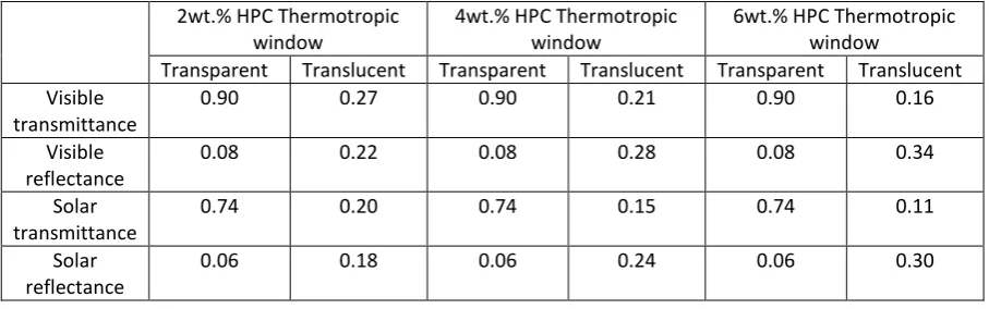
8 4.1 Measurement data
2
The measured transmittance and reflectance values for the three types of thermotropic
3
window are shown in Table 3. From these data it can clearly be seen that in its transparent
4
state, transmittance and reflectance values are identical for all concentrations. Indeed if
5
considering the properties outlined in Table 3, solar transmittance is similar to that of a
6
conventional double glazed unit (0.79 for ODG, 0.74 for TT). However when the HPC has
7
transitioned into its translucent state, higher concentrations lead to lower transmittance
8
and conversely increased reflectance, ranging from a solar transmittance of 0.20 at 2wt.%
9
concentration to 0.11 at 6wt.%. In the case of the 6wt.% HPC concentration, solar
10
transmittance is in the order of 5x less than that of a solar controlled low-e coated glazing
11
unit. As a result, at higher HPC concentrations, one can expect considerably more rejection
12
of solar heat gain in the transitioned state.
[image:8.595.66.520.295.437.2]13 14
Table 3 - Measured optical properties of the developed thermotropic smart window
15
2wt.% HPC Thermotropic window
4wt.% HPC Thermotropic window
6wt.% HPC Thermotropic window
Transparent Translucent Transparent Translucent Transparent Translucent Visible
transmittance
0.90 0.27 0.90 0.21 0.90 0.16
Visible reflectance
0.08 0.22 0.08 0.28 0.08 0.34
Solar transmittance
0.74 0.20 0.74 0.15 0.74 0.11
Solar reflectance
0.06 0.18 0.06 0.24 0.06 0.30
16 17
4.2 Effect of window inclination, glazing type and HPC concentration on loads and energy 18
performance 19
The four window inclinations as shown in Figure 2 were tested for all glazing combinations
20
using EnergyPlus to explore their overall performance in relation to heat gains, heating,
21
cooling and lighting loads and ultimately overall building energy consumption.
22 23
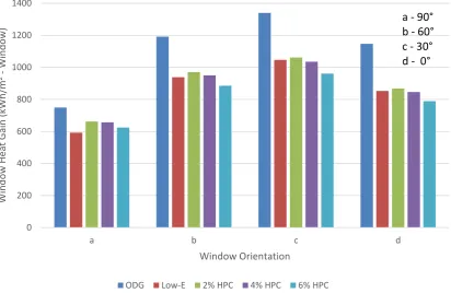
4.2.1 Window heat gain 24
Figure 3 shows the window total heat gains of each window type for each discrete plane
25
inclination; a - 90°, b - 60°, c -30° and d - 0° to the horizontal. As would be expected, the
26
ODG unit, with its higher solar transmittance consistently has the highest window heat gain
27
irrespective of plane inclination. However with respect to the other glazing types, the
28
ordering as a function of total heat gain changes in response to plane inclination. At 60o
29
inclination, LE glazing outperforms all but the 6wt.% TT unit but this changes as plane
30
inclination reaches 30o and 0o to the horizontal where the 4 wt.% concentration begins to
31
show an improvement over the LE unit. It can be seen therefore that with a decrease in roof
32
gradient, TT windows with higher HPC concentrations begin to show their effectiveness over
33
LE glazing. This can be explained due to the higher solar altitude for this particular latitude,
34
where those windows with a lower inclination angle (i.e. moving towards the horizontal) are
9
more exposed to increased incident solar radiation which in turn allows the window to
1
maintain a higher temperature for a longer period of time. By being at or above Ts for
2
longer, the windows are in their translucent state for a greater period of the day thus
3
rejecting incoming solar radiation. This dynamic fluctuation between transparent and
4
translucent states for HPC-based TT windows therefore positively benefits control over solar
5
heat gain when compared to the static behaviour of LE glazing units.
6
This behaviour can clearly be seen when inspecting the data from the 6wt.%
7
concentration and comparing it to the LE coated unit. In its transparent state, the HPC unit
8
has a solar transmittance of 0.74 and in its translucent state this is 0.11. The LE unit
9
however has a fixed transmittance of 0.53. During cooler periods the lower solar
10
transmittance of the LE unit reduces beneficial solar gains into the space and in turn impacts
11
on passive solar heating thus potentially increasing its heat load. Conversely, during warmer
12
periods, the lower transmittance of the HPC unit reduces detrimental gains. This is also
13
mirrored in the solar reflectance data. With a fixed reflectance of 0.22, the LE coated unit
14
rejects more incoming gains in cooler periods in comparison to the HPC unit (0.06). When
15
transitioned, the HPC unit has a solar reflectance of 0.30, 0.08 higher than the static
16
performance of the LE unit. More incoming radiation is therefore rejected by the HPC unit
17
during warmer spells.
18
When comparing across the thermotropic glazing variants, figure 3 clearly shows that TC
19
windows with higher concentrations of HPC have the lowest heat gain. Having transitioned
20
into their translucent state, solar transmittance at 6wt.% concentration is approximately
21
half that at 2wt.% concentration (0.11 at 6wt.%, 0.22 and 2wt.%). This is this mirrored in the
22
solar reflectance values which increase significantly based on concentration strength (0.18
23
at 2wt.% to 0.30 at 6 wt.%)
10 1
Figure 3 – Total annual window heat gain for the different glazing combinations at varying plane inclination
2
angles
3
4
4.2.2 Room Heating/Cooling and Lighting Loads 5
Figure 4 shows the annual energy consumption of each window type for each of the four
6
discrete orientations. For clarity and as mentioned in section 3.2, to account for volumetric
7
differences in each model tested, the overall energy consumption has been standardised to
8
kWh/m3, where this includes the heating / cooling and lighting loads for the office space.
9
As with the results from 4.2.1, the data clearly shows the interrelationship between solar
10
altitude, plane inclination and glazing type and its impact on total energy consumption. A
11
close inspection of Figure 4 shows that in all cases, lighting loads increase as a function of
12
glazing type; that is ODG has the lowest lighting load due to its lower visible light
13
transmittance, this peaking where the HPC concentration is set at 6wt.%. When considering
14
heating demand data for this particular latitude, an almost identical trend across all plane
15
inclinations appears. In all cases, annual heating demand is lowest for ODG due to it
16
receiving beneficial solar gains. HPC concentrations of 2 wt.% and 4wt.% result in almost
17
identical heating demands at each plane inclination and have the next lowest demand and
18
similarly, both LE and HPC glazing at 6wt.% concentrations have almost identical heating
19
demands at all plane inclinations. When combined with the cooling load data, an interesting
20
trend emerges that reinforces the conclusions from section 4.2.1. As expected, cooling load
21
is greatest at all plane inclinations for the ODG unit; a product of its high solar transmittance
22
and therefore high heat gains. Very little difference in cooling loads can be observed
23
between HPC concentrations of 2wt.% and 4wt.%. However the effects of solar altitude and
24
switching / transition behaviour can be observed when closely inspecting the LE and 6wt.%
25
0 200 400 600 800 1000 1200
a b c d
Win
d
o
w
H
eat
Gain
(k
Wh
/m
2
Win
d
o
w
)
Window Orientation
ODG Low-E 2% HPC 4% HPC 6% HPC
11
glazing data. Here, LE glazing outperforms the 6wt.% concentration by approximately
1
3kWh/m3 annually for a vertical plane (90o). However the benefits of the increased HPC
2
concentration can be seen as the inclination angle reduces. At 60o inclination, cooling loads
3
are almost identical at approximately 28.3 kWh/m3 however by the time the plane reaches
4
0o inclination (horizontal plane), the 6wt.% HPC-based TT unit outperforms the LE unit by
5
approximately 4kWh/m3 annually.
6
It is important that both heating and cooling load data are viewed with respect to
7
the thermal transmittance (U) values of the HPC-filled units in relation to the LE unit.
8
Indeed, for the purpose of these simulations, the U-value of the LE unit (1.7 W/m2K) was 1
9
W/m2K lower than the HPC units (2.7 W/m2K). In the specific case of the 6wt.% HPC unit at
10
60o, its heating and cooling performance was almost identical to that of the LE unit
11
irrespective of the lower thermal transmittance of the LE unit, its performance improving as
12
plane inclination decreased.
13
When viewed overall, it is evident that at high inclination angles (e.g. 90o) for this
14
particular latitude, HPC-based TC windows receive less incident radiation and therefore
15
cannot maintain a high enough temperature to transition. This is evident in the virtually
16
identical heating and cooling load data for all three HPC concentrations suggesting that the
17
glazing itself has not transitioned to a translucent state. As the window’s inclination
18
decreases from 90o to 0o, the TT windows begin to show their energy saving potential over
19
both ODG and LE glazing units. In this case, one can see the benefit of the glazing units
20
switching between transparent and translucent states and the resultant rejection to
21
incoming solar radiation. As the plane approaches 0o inclination, its transition is maintained
22
for a longer period of time due to its relationship with solar altitude and associated heat
23
gains and here we can see the true benefit of the higher HPC concentration over other
24
glazing variants.
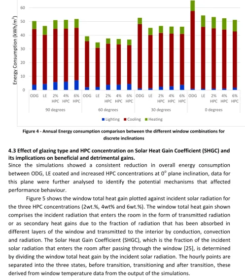
12 1
Figure 4 - Annual Energy consumption comparison between the different window combinations for
2
discrete inclinations
3
4.3 Effect of glazing type and HPC concentration on Solar Heat Gain Coefficient (SHGC) and 4
its implications on beneficial and detrimental gains. 5
Since the simulations showed a consistent reduction in overall energy consumption
6
between ODG, LE coated and increased HPC concentrations at 0o plane inclination, data for
7
this plane were further analysed to identify the potential mechanisms that affected
8
performance behaviour.
[image:12.595.55.553.95.656.2]9
Figure 5 shows the window total heat gain plotted against incident solar radiation for
10
the three HPC concentrations (2wt.%, 4wt% and 6wt.%). The window total heat gain shown
11
comprises the incident radiation that enters the room in the form of transmitted radiation
12
or as secondary heat gains due to the fraction of radiation that has been absorbed in
13
different layers of the window and transmitted to the interior by conduction, convection
14
and radiation. The Solar Heat Gain Coefficient (SHGC), which is the fraction of the incident
15
solar radiation that enters the room after passing through the window [25], is determined
16
by dividing the window total heat gain by the incident solar radiation. The hourly points are
17
separated into the three states, before transition, transitioning and after transition, these
18
derived from window temperature data from the output of the simulations.
19
As can be seen from Table 4, in their transparent state, all HPC concentrations have a
20
SHGC of 0.56. This is a small improvement over the static SHGC for LE glazing (0.54) but
21
considerably less than that of an ODG unit (0.74). It can therefore be expected that
22
considerably more desirable gains will arise from an ODG unit during cooler periods (i.e.
23
when the TT units have not transitioned). However having transitioned to their translucent
24
state due to higher temperatures or stronger irradiance, all TT HPC concentrations have a
25
0 10 20 30 40 50 60
ODG LE 2%
HPC 4% HPC
6% HPC
ODG LE 2%
HPC 4% HPC
6% HPC
ODG LE 2%
HPC 4% HPC
6% HPC
ODG LE 2%
HPC 4% HPC
6% HPC
90 degrees 60 degrees 30 degrees 0 degrees
Lighting Cooling Heating
Energ
y C
o
n
sump
tio
n
(kW
h
/m
13
considerably lower SHGC than their LE coated or ODG counterparts (0.50 at 2wt.%, 0.47 at
1
4wt.%, 0.44 at 6wt.%). As such, with a decreasing SHGC, the ability for the window to
2
minimise undesirable heat gain increases at increased HPC concentrations due to their
3
lower solar transmittance and higher solar reflectance. It seems therefore that the switching
4
behaviour of the unit is a positive asset over conventional ODG or LE units, where dynamic
5
control is exerted over incoming gains. The true benefits (or detriments) to passive heating
6
or cooling however must be seen in light of the differences in thermal transmittance
7
between the various units.
14 1
2
Figure 5 - Window Solar Heat Gain Coefficients for the 2, 4 and 6wt.% HPC Thermotropic (TT) Windows
3
0 100 200 300 400 500 600 700
0 100 200 300 400 500 600 700 800 900 1000
2wt.% HPC TT Window
0 100 200 300 400 500 600 700 800
0 100 200 300 400 500 600 700 800 900 1000
Incident Solar Radiation (W/m2 - Window)
Before Transition Transitioning After Transition
ODG - SHGC Low-E - SHGC
6wt.% HPC Window
Win
d
o
w
Tot
al
H
eat
Gain
(W/m
2
Win
d
o
w
)
Avg SHGC Before Avg SHGC After Transition
0 100 200 300 400 500 600 700 800
0 100 200 300 400 500 600 700 800 900 1000
15
Table 4 – Solar Heat Gain Coefficients for the three HPC concentrations
1
HPC Concentration SHGC (Transparent State) SHGC (Translucent State)
2% 0.56 0.5
4% 0.56 0.47
6% 0.56 0.44
2
4.4 Detailed Analysis of Horizontal Roof with 6 wt.% HPC TT window Installed 3
Since the performance of the HPC-based thermotropic window is influenced by a
4
combination of various environmental conditions, the effects of air temperature and
5
incident solar radiation on the temperature of the thermotropic layer and window total
6
heat gains were explored for a representative 3 days period during both heating and cooling
7
seasons for the 6wt.% HPC concentration. This HPC TC concentration consistently showed
8
improved performance over all HPC glazing variants and hence was used for further study.
9
In so doing, the combination of outdoor temperature and incident solar radiation resulting
10
in thermotropic layer temperatures high enough to cause light scattering were considered in
11
addition to the corresponding window heat gains. These data were considered with respect
12
to both ODG and LE glazing units.
13 14
4.4.1 Temperatures, Incident Radiation and Window Heat Gain 15
Figure 6a shows the outdoor and indoor temperatures experienced during the
16
representative 3 day period in winter and summer with the use of a HVAC system for a
17
window inclination of 0°. Temperatures for the thermotropic layer are also plotted with
18
corresponding incident solar radiation and window heat gains attributed to each test
19
window type.
20
In Palermo the outdoor temperature during the heating season ranges between 6-12°C
21
while the indoor temperature in every simulation is maintained at a constant temperature
22
of 22°C by the HVAC system heating the room. Although in the simulations on each window
23
type the incident solar radiation will be the same, the simulated window heat gains are
24
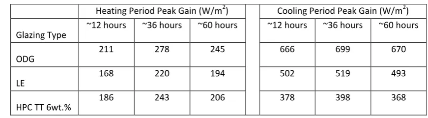
different. As can be seen from Figure 6b and Table 5, the use of solar control LE glazing
25
reduces the peak window heat gain by approximately 20.7% in comparison with an ODG
26
unit during the representative heating period, while the 6wt.% HPC TT window reduces the
27
heat gain by approximately 13.4%. The peaks in window heat gains correspond directly to
28
the peaks in incident solar radiation and therefore window temperatures, clearly identifying
29
that the windows had not reached their switching temperature therefore drawing a strong
30
link between amount of incident solar radiation and ability for the thermotropic window to
31
transition.
32
Given that during the heating period, any reduction in window heat gain may be
33
undesirable as it reduces the potential for passive solar heating, the static nature of solar
34
controlled LE windows has a constant and negative effect on solar heat gains in comparison
35
to both ODG and HPC-based TC units, although its true effect from an energy consumption
36
perspective will be mitigated by its improved thermal transmittance values.
16
indoor temperature again being maintained by the HVAC system cooling the room. Unlike in
2
the heating period simulation, the TC window heat gains are now reduced further than
3
those of the solar control LE window. Both LE and HPC TT glazing units show considerable
4
reductions in peak heat gains over the ODG unit at 25.6% and 43.8% respectively during the
5
representative cooling period. When comparing the HPC TT to the LE unit, the HPC TT unit
6
reduces total heat gains by 24.5%. As expected, the peaks in incident radiation correspond
7
to the peaks in window heat gain and TT layer temperature. As can be seen from Figure 6a,
8
in the cooling period, the TT layer temperatures exceed 60°C at midday ensuring transition
9
of the layer, therefore the space below can take advantage of the solar shading potential of
10
this unit. In total, the TT window layer is in its translucent / reflective state for
11
approximately 21 out of 72 hours during the designated simulation period. In this time, the
12
TT glazing unit has a SHGC of 0.44 as compared to a static SHGC of 0.54 for the LE or 0.74 for
13
ODG glazing units. The potential for savings on cooling energy that arise from solar heat
14
gains are therefore evident.
[image:16.595.75.511.349.469.2]15
Table 5 – Total heat gains for the three window types
16
Heating Period Peak Gain (W/m2) Cooling Period Peak Gain (W/m2) Glazing Type ~12 hours ~36 hours ~60 hours ~12 hours ~36 hours ~60 hours
ODG 211 278 245 666 699 670
LE 168 220 194 502 519 493
HPC TT 6wt.% 186 243 206 378 398 368
17 1
Figure 6 (a) Ambient temperatures and thermotropic layer temperature for heating and cooling period,
2
(b) Incident solar radiation and window total heat gain for heating and cooling period
3
4
0 10 20 30 40 50 60 70
0 12 24 36 48 60 720 12 24 36 48 60 72
Tem
p
e
ratu
re
(
°C)
Heating Period Cooling Period
Hours into Simulation (hrs)
Outdoor Temperature Indoor Temperature 6% HPC Layer Temperature
(a)
0 100 200 300 400 500 600 700 800 900
0 12 24 36 48 60 720 12 24 36 48 60 72
So
lar
R
ad
iation
/ To
tal H
e
at
Gai
n
(
W/m
2
Wi
n
d
o
w)
Heating Period Cooling Period
Hours into Simulation (hrs)
Incident Solar Radiation ODG Window Total Heat Gain
Low-E Window Total Heat Gain 6% HPC Window Total Heat Gain (b)
Day 1 Day 2 Day 3 Day 1 Day 2 Day 3
[image:17.595.69.509.73.717.2]18
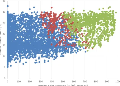
It is known that there is a strong correlation between switching response to both outdoor
2
air temperature and incident solar radiation [7]. This is evident in Figure 7 which shows
3
hourly sets of data for outdoor air temperature plotted against solar radiation incident on
4
the glazing, these acquired through an annual simulation. The 6 wt.% HPC TT window is in
5
its translucent state for approximately 1056 hrs of the annual (8760 hrs) simulation. In
6
addition, it spends approximately 396 hrs in transition. Although the outdoor temperature
7
never approaches the transition range of 40-50°C the combination of outdoor temperature
8
and incident solar radiation results in the HPC membrane transitioning to its translucent /
9
reflective state. Simulation results show that transitioning takes place between the months
10
of March and October for this location and highlights the three transition phases (Figure 7):
11
(1) the window is transparent when the incident solar radiation is less than approximately
12
300 W/m2 at temperatures lower than 30oC. (2) The transition phase itself occurs at solar
13
radiation intensities greater than 300 W/m2 and for temperatures higher than 14oC. (3) For
14
lower solar radiation intensities, i.e. at approximately 500W/m2, transition to the
15
translucent state takes place at air temperatures around 20oC, where the required air
16
temperature reduces as solar radiation intensity increases.
17 18
[image:18.595.97.504.381.673.2]19
Figure 7 - The state of the HPC layer under combination effects of irradiation and outdoor ambient
20
temperature
21
0 5 10 15 20 25 30 35
0 100 200 300 400 500 600 700 800 900 1000
Ou
td
o
o
r
Te
m
p
era
tu
re
(
°C)
Incident Solar Radiation (W/m2 - Window)
19
To explore the impact of incident solar radiation on the 6wt.% HPC layer temperature, the
1
data were further analysed, the results presented in Figure 8. As can be seen, the HPC layer
2
temperature increases in direct proportion to incident solar radiation. The HPC layer
3
reaches a maximum temperature of 70°C with an incident solar radiation intensity of
4
approximately 1000W/m2, confirming the assumption that although the outdoor
5
temperature may be much lower than the transition temperature range, the added heat
6
provided by the incident solar radiation pushes the HPC layer temperature into the
7
transition range. As the HPC layer is sandwiched between two glazing panels, this design
8
helps to decouple the HPC layer from the indoor thermal environment and any unwanted
9
effects this would have.
10
[image:19.595.94.504.263.545.2]11
Figure 8 - The effect of irradiation on the HPC layer temperature
12
4.4.3 Window Heat Gain and Incident Solar Radiation 13
Building upon the analysis from section 4.3, Figure 9 shows the window total heat as a
14
function of incident solar radiation. The inherent changeability of the 6wt.% HPC TT window
15
results in a range of SHGCs that depend on the state of the window with two transition
16
states (before and after) clearly evident from the graph. Before transitioning, the SHGC is
17
0.56 and post transition it is 0.44. The transitioning points appear split in this way as the first
18
group is made up of points attempting to transition predominantly due to high levels of
19
incident radiation while the second group is made up of points attempting to transition
20
predominantly due to high ambient temperatures; when both factors are present the
21
0 10 20 30 40 50 60 70 80
0 200 400 600 800 1000 1200
TT
La
ye
r
Te
m
p
era
tu
re
(C
)
Incident Solar Radiation (W/m2 - Window)
20
solar radiation and window total heat gains. However what is slightly more ambiguous is the
2
SHGC during transition which very much depends on the combinations of incident solar and
3
ambient temperature.
4
[image:20.595.65.515.155.452.2]5
Figure 9 – Sets of hourly external incident radiation and window total heat gain through a year
6
4.4.4 Heat Gain/Loss through windows 7
Monthly Simulations 8
Figure 10 shows the monthly heat gains/losses for the Double Glazing (ODG), solar control
9
Low-E (LE) and 6wt.% HPC TT window combinations. Unlike the heat gains, the heat losses
10
are primarily caused by the conductive, convective and radiative heat transfer processes
11
between the indoor and outdoor environment, these dominated by the thermal
12
transmittance (U-value) of the glazing unit. The thin HPC layer does not significantly affect
13
this u-value and this is evident when comparing the losses for both the ODG and TT units
14
which have identical U-values (2.7W/m2K). Improvements in heat loss performance can
15
however be seen with the LE unit that has a considerably lower U-value of 1.7 W/m2K.
16
With respect to heat gains, the figure clearly shows that there is a defined transition
17
point where the performance of the LE and HPC-based TT units cross in both March and
18
October. That is, at some point during these two months, the HPC-based TT unit begins to
19
match the overall thermal performance of the LE unit, irrespective of the differences in
U-20
values. As can be seen from the figure, during the heating period (i.e. from October until
21
March), the ODG unit’s high solar transmittance results in higher (beneficial) solar gains.
22
With the lowest solar transmittance, the LE unit results in the lowest beneficial solar gains.
23
y = 0.5646x - 4.58
y = 0.4429x - 9.022
0 100 200 300 400 500 600 700 800
0 100 200 300 400 500 600 700 800 900 1000
Win
d
o
w
Tot
al
H
eat
Gain
Ra
te (W/m
2
Win
d
o
w
)
Incident Solar Radiation (W/m2 - Window)
Before Transition Transitioning After Transition
21
However from March until October, the TT unit shows a marked reduction in overall gains
1
over its LE counterpart, showing the importance of the switching / transition point in
2
helping to control unwanted solar gains.
3
[image:21.595.42.552.129.682.2]4
Figure 10 – Monthly window heat gains/losses comparison between ODG, LE and 6% HPC TT
5
Annual Simulations 6
Figure 11 shows the annual heat gains/losses through windows for the different window
7
types. Overall, the TT window had the largest reduction in annual solar heat gain of the
8
three glazing systems. In comparison with ODG, the LE unit reduces heat gains by
9
approximately 26% or 294kWh/m2 (through window). Additionally, it reduces heat losses by
10
approximately 33% or 41kWh/m2 when compared to ODG. The TT reduced heat gains by
11
31% or 358kWh/m2 (when compared to ODG. From Figures 10 and 11, it can be seen that
12
the TT window provides larger benefits than the LE window during the cooling period. As
13
heat gains are predominantly due to incident solar radiation during this period this shows
14
that the TT window’s translucent and reflective state has taken effect. The solar control LE
15
window appears more beneficial during the heating period, however, as heat losses are
16
predominantly affected by the thermal transmittance (U-value) of the glazing unit and
17 reduced emissivity. 18 19 0 20 40 60 80 100 120 140 160 180 O D
G LE TT
O
D
G LE TT
O
D
G LE TT
O
D
G LE TT
O
D
G LE TT
O
D
G LE TT
O
D
G LE TT
O
D
G LE TT
O
D
G LE TT
O
D
G LE TT
O
D
G LE TT
O
D
G LE TT
Win d o w H eat Gain /Lo ss (kWh /m
2
Win
d
o
w
)
Heat Gain Heat Loss
[image:21.595.76.551.139.412.2]22 1
Figure 11 - Annual window heat gains/losses comparison between ODG, LE and 6% HPC TT
2 3
4.4.5 Room Heating/Cooling and Lighting Loads 4
Monthly Simulations 5
Figure 12 shows the monthly room heating/cooling loads as well as the attributed lighting
6
loads. Although a decreased HVAC load is important, a whole system view must be taken to
7
fully understand the energy implications of the alternate window choices. As can be seen,
8
for this particular building type, cooling dominates from March to November and the
9
benefits of the HPC-based TT unit can be seen from April until September. For example, in
10
the month of July, the LE window reduces the cooling load by approximately 19% compared
11
with the ODG, while the TT window reduces the cooling load by 28%. A close inspection of
12
the data however shows that for the entire year, artificial lighting is required for the
HPC-13
based TT unit in order to reach the minimum of 500 lux within the office. For example, in
14
the same July period, both the ODG and LE unit require no artificial lighting whereas the TT
15
unit requires 0.25 kWh/m2 as the glazing unit will have switched from its transparent to
16
translucent state for a significant period of the working day lowering the visible
17
transmittance to 0.16. However in the case of the ODG and LE units, artificial lighting is only
18
required between the months of October and February, with the higher visible
19
transmittance of the ODG unit requiring less lighting energy. It can clearly be seen therefore
20
that the benefits of the TT unit are somewhat mitigated by the increased energy
21
consumption that arises due to lighting loads and any additional cooling demand that will be
22
placed due to these loads. It is however evident in the round that the TT unit does give rise
23
to lower energy demands overall during the cooling period.
24 25 26
0 200 400 600 800 1000
ODG LE TT
Win
d
o
w
H
eat
Gain
/Lo
ss
(kWh
/m
2
Win
d
o
w
)
23
[image:23.595.84.505.79.356.2]
1
Figure 12 - Monthly Heating/Cooling and Lighting Load comparison between ODG, LE and 6wt.% HPC TT
2
Annual Simulations 3
Table 6 and Figure 13 show the annual heating/cooling and lighting loads for the office with
4
different window types installed. From Figure 13, it can be seen that there are no
5
substantive differences in annual lighting loads between ODG and LE units. This is not true
6
for the TT unit however which requires in the order of 80% more lighting energy to reach
7
the required illuminance levels. Proportionally however there is little substantive difference
8
in heating loads between the three glazing types. The main difference can be seen in cooling
9
loads where a 6wt.% HPC-based TT unit will reduce overall annual cooling requirements by
10
27.7% over an ODG unit and by 9.9% over a LE unit for this particular example. Overall this
11
translates to total energy savings of approximately 22% over ODG and 6% over LE coated
12
units. This must be seen with respect to potential issues surrounding daylight availability
13
and the associated health and wellbeing consequences that arise due to this which are a
14
product of the reduced visible transmittance of the unit in its transitioned state.
15 16 17 18 19 20 21 22 23 24 25
0 5 10 15 20 25 30 35
OD
G LE TT
OD
G LE TT
OD
G LE TT
OD
G LE TT
OD
G LE TT
OD
G LE TT
OD
G LE TT
OD
G LE TT
OD
G LE TT
OD
G LE TT
OD
G LE TT
OD
G LE TT
H
eat
in
g/C
o
o
ling/L
ight
in
g
Lo
ad
s (k
Wh
/m
2
Floo
r)
Heating Load Cooling Load Lighting Load
24
Energy Consumption kWh/m2 PA
Load ODG LE 6wt.% TT
Lighting 2.96 3.05 5.43
Cooling 170.16 135.25 123.04
Heating
22.78 24.95 25.06
Total 195.9 163.25 153.53
2
[image:24.595.59.510.64.591.2]3 4
Figure 13 - Annual Heating/Cooling and Lighting loads comparison between ODG, LE and 6wt.% HPC TT
5
6
7
8
0 20 40 60 80 100 120 140 160 180 200
ODG LE TT
H
eat
in
g/C
o
o
ling/L
ight
in
g
Lo
ad
s (k
Wh
/m
2
Floo
r)
25 4.5 Effect of Transition Temperature for a Horizontal Roof with 6 wt.% HPC TT Window 1
Installed 2
3
The final suite of simulations sought to explore the impact of transition temperature (Ts) on
4
overall performance, particularly with respect to window total heat gains, solar heat gain
5
coefficients and annual energy consumption. Studies to date have shown that the addition
6
of sodium chloride to the HPC mixture can work to reduce this range [17]. As such, using the
7
original spectral data but applying it to lowered transition temperatures, predictions were
8
carried out for transition temperatures of 35 - 45°C, 30 - 40°C, 25 - 35°C, and 20-30°C.
9 10
4.5.1 Heat Gain through window 11
Figure 14 shows the total heat gains through a 6wt.% HPC-based TT window subject to
12
varying transition temperatures. These are compared to the total heat gains of ODG and
13
solar control LE windows. It can be seen that reducing the transition temperature from
40-14
50oC to 20-30oC reduces the overall annual window heat gain by 147kWh/m2. When
15
compared to ODG and LE units, gains are reduced by 505.6 and 211.3 kWh/m2 respectively
16
representing annual reductions of 44% and 24.7% respectively.
17
[image:25.595.92.503.353.624.2]18
Figure 14 – Annual Window Total heat Gain comparison between the different windows and
19
transition temperature ranges
20 21
As the transition temperature range decreases, the TT window is able to enter its
22
translucent / reflective state for longer periods of time therefore decreasing both solar and
23
visible light transmittance for extended periods. Whilst this might be beneficial from the
24
perspective of cooling loads, this has to be offset against both the additional heating
25
demands of the building during the heating period and the associated lighting demands
26
1,146.96
852.71
788.50
735.40
690.35
659.56 641.37
0 200 400 600 800 1000 1200
ODG Low-E 40-50 35-45 30-40 25-35 20-30
H
eat
Gain
t
h
ro
u
gh
wind
o
w
(k
jW
h
/m
2
Win
d
o
w
)
26
state.
2 3
4.5.2 Window Heat Gain and Incident Solar Radiation 4
The SHGC of the 6wt.% HPC TT has been explored in depth in section 4.4. This section will
5
look at the SHGCs of the five transition temperature ranges of the 6wt.% HPC TT. In so
6
doing, it compares these transition temperatures against each other and also with the ODG
7
and LE test windows. Figure 15 shows the window total heat gain plotted against incident
8
solar radiation for the five transition temperature ranges of the 6wt.% HPC TT. The hourly
9
points are separated into the three states: before transition, transitioning and after
10
transition.
11
As discussed previously, the average range of the SHGC for a 6wt.% HPC TT with the
12
original 40-50°C transition temperature range, is approximately 0.44 – 0.56, this a product
13
of the TT’s ability to change its spectral properties. The average range of the SHGC for
14
transition ranges of 35 - 45°C HPC TT and for 30 – 40°C TT are also 0.44 - 0.56. Although the
15
transition temperature has changed, the optical characteristics remain constant, however,
16
with lower transition temperatures the number of translucent hours increases.
17
When the transition temperature range falls to 25-35°C and 20-30°C, in the Palermo
18
climate, the number of translucent hours greatly increases resulting in the SHGC becoming a
19
single average value; the SHGC for 25 – 35°C and 20 – 30°C HPC TT are both 0.44 on
20
average. In other words, the window has transitioned to its translucent state for a
21
significant period across the year. This coefficient falls below that of even the solar
22
controlled LE window (0.54), meaning that during the cooling period, the solar heat gain
23
through the window is reduced further by the use of the TT window. However during the
24
heating period this configuration reduces passive solar heating significantly which may be
25
undesirable.
26 27
27 1
0 100 200 300 400 500
0 100 200 300 400 500 600 700 800 900 1000
Incident Solar Radiation (W/m2 - Window)
Before Transition Transitioning After Transition
ODG - SHGC Low-E - SHGC SHGC Avg
Avg SHGC Before Transition Avg SHGC After Transition
0 100 200 300 400 500
0 100 200 300 400 500 600 700 800 900 1000
0 100 200 300 400 500
0 100 200 300 400 500 600 700 800 900 1000
0 100 200 300 400 500
0 100 200 300 400 500 600 700 800 900 1000
0 100 200 300 400 500
0 100 200 300 400 500 600 700 800 900 1000
[image:27.595.92.511.80.722.2]Transition range 20-30°C
Figure 15 – Window Solar Heat Gain Coefficients for the different transition temperature ranges
Transition range 25-35°C
Transition range 30-40°C
Transition range 35-45°C
Transition range 40-50°C
Win
d
o
w
Tot
al
H
eat
Gain
(W/
m
2 –
Win
d
o
w