The development and assessment of cardiac magnetic resonance imaging for the detection of age and disease related changes in the human heart

MAGNETIC RESONANCE IMAGING FOR THE DETECTION OF AGE- AND DISEASE-RELATED CHANGES IN THE

HUMAN HEART

Shona Matthew

A Thesis Submitted for the Degree of PhD at the

University of St Andrews

2012

Full metadata for this item is available in Research@StAndrews:FullText

at:

http://research-repository.st-andrews.ac.uk/

Please use this identifier to cite or link to this item: http://hdl.handle.net/10023/3558

This item is protected by original copyright

Resonance Imaging for the Detection of Age- and

Disease-Related Changes in the Human Heart

Shona Matthew

This thesis is submitted in partial fulfilment for the

degree of PhD at the University of St Andrews

This thesis is dedicated to my foster parents

Frank & Mary Dow

and

Christine & Jimmy Craig

Abstract and scope i

Abstract i

The Scope of the Thesis ii

Acknowledgements vi

Significant events in the history of NMR and MRI 2

1. The Basics of MRI 3

1.1 Diagnostic Imaging 4

1.2 Magnetic Resonance Imaging 4

1.3 Nuclear Magnetic Resonance 5

1.4 Spin Angular Momentum 5

1.4.1 Gyromagnetic Ratio 6

1.5 Hydrogen Nuclei 7

1.6 The Zeeman Effect 7

1.7 The Boltzmann Distribution 8

1.8 Larmor Equation 9

1.9 Net Magnetisation Vector 9

1.10 The Main Magnetic Field 11

1.10.1 Superconducting Magnets 11

1.11 The Radio Frequency Field 12

1.12 Resonance 13

1.12.1 Rotating Frame of Reference 13

1.12.2 Flip Angles 14

1.12.3 Partial Flip Angles 15

1.12.4 Free Induction Decay 15

1.12.5 T1 Relaxation 16

1.12.6 T2 Decay 17

1.12.7 T2* Relaxation 18

1.13 Image Formation 19

1.13.1 Gradient Magnetic Fields 20

1.13.2 Slice Select Gradient 20

1.13.3 Frequency Encoding 21

1.13.4 Phase Encoding 22

1.13.5 Repetition Time 24

1.13.6 Echo Time 25

1.13.7 Biological Parameters 25

1.14 Pulse sequences 25

1.14.1 Spin Echo 26

1.14.2 Spin Echo – T1 Weighted Images 27

1.14.3 Spin Echo – T2 Weighted Image 27

1.14.7 Pathology Scans 31

1.14.8 Proton Density Scans 31

1.15 Coils 32

1.15.1 Body Coil 32

1.15.2 Shim Coil Sets 32

1.15.3 Surface Coils 33

1.15.4 Phased Array Coils 33

1.16 K-Space 34

1.17 SAR limitation 38

1.18 Cardiac Magnetic Resonance Imaging 39

1.19 Other Techniques and their Limitations 40

1.19.1 SPECT and PET 40

1.19.2 Computed Tomography 41

1.19.3 Echocardiography 42

1.20 The Advantages of Cardiac Magnetic Resonance Imaging 43 1.21 The Limitations of Cardiac Magnetic Resonance Imaging 44

References 46

2. The Human Heart 49

2.1 The Chambers of the Heart 50

2.2 The Valves of the Heart 51

2.3 The Papillary Muscles 52

2.4 The Myocardium 53

2.5 Path of Blood through the Heart 54

2.6 The Coronary Arteries 56

2.7Blood Pressure 56

2.8 The Cardiac Cycle 57

2.9 The Electrocardiogram 57

2.10 Diseases of the Heart 58

2.10.1 Coronary Artery Disease 58

2.10.2 Valve Disease 60

2.10.3 Left Ventricular Hypertrophy 61

2.10.4 Cardiac Arrhythmias 62

2.10.5 Heart Failure 62

2.11 Acknowledgments 63

References 64

3. The Development of Cardiac Magnetic Resonance Imaging 66

3.1 Hardware Developments 67

3.1.1 Higher Fields 67

3.1.2 Gradient Capabilities 68

3.1.3 Phased Array Coils 69

3.1.4 Parallel Imaging 71

3.2.3 Echo Planar Imaging 75

3.3 Cardiac Applications 76

3.3.1 Breath-Holding Techniques 76

3.3.2 Gating and Triggering Techniques 76

3.3.2.1 Prospective Triggering 77

3.3.2.2 Retrospective Gating 77

3.4 Contrast Agents 78

3.5 Conclusion 79

References 80

4. The Advantages, Challenges and Limitations of Imaging at 3.0T in Comparison

to 1.5T 83

4.1 Introduction 83

4.2Technical Details of the Magnetic Fields 84

4.3 The Images 84

4.4 The Signal 85

4.5 The Noise 86

4.5.1 Signal-to-Noise Ratio 87

4.6 The Advantages of CMRI at 3.0T 88

4.7 The Challenges and Limitations of CMRI at 3.0T 89

4.7.1 Chemical Shift 89

4.7.2 Chemical Shift of the Second Kind 92

4.7.3 Dielectric Effect 94

4.7.4 B1 Inhomogeneities 94

4.7.5 Changes in Power Deposition and the Impact on SAR limitations 95 4.7.6 FieldInhomogeneities and Susceptibility 97

4.7.7 Susceptibility Effects 98

4.7.8 Metal Artefact 99

4.7.9 Shimming 100

4.7.10 Parallel imaging 101

4.7.11 Coils 102

4.7.12 The Magnetohydrodynamic Effect 102

4.7.13 Vector Cardiogram 103

4.7.14 Contrast to Noise Ratio 104

4.8 The Changes in Tissue Relaxation Times 104

4.9 Contrast Enhancement 105

5. Cardiac Magnetic Resonance Imaging Protocols 106

5.1 Introduction 106

5.2 Fast Gradient Echo 106

5.3 TrueFISP 107

5.3.1 Equilibrium 107

5.3.5 Optimal Flip Angle 111

5.3.6 Optimal Signal 111

5.3.7 Artefacts 112

5.4 TurboFLASH 113

5.5 The Images 113

5.5.1 Reference Images 113

5.5.2 The Localisers 113

5.6 Functional Imaging 116

5.6.1 Clinical Information 117

5.7 First Pass Perfusion Imaging 118

5.7.1 Clinical Information 119

5.8 Post Processing of Cardiac Images 119

5.8.1 Cardiac Volumes 119

5.8.2 Cardiac Mass 119

5.8.3 Cardiac Output and Ejection Fraction 120

References 121

6. Assessment of clinical differences at 1.5T between quantitative right and left

ventricular volumes and ejection fractions using MRI 122

6.1 Introduction 122

6.2 Aims 122

6.3 Cohorts 123

6.4 Acquisition Protocol 124

6.5 Image Analysis 124

6.6 Statistical Analysis 125

6.7 Results 126

6.8 Discussion 129

6.8.1 Reproducibility 129

6.8.2 Significant Changes in Cardiac Parameters 130

6.9 Conclusion 130

References 131

7. Normal Ranges of Left Ventricular Functional Parameters at 3 Tesla 132

7.1 Part 1 132

7.2 The Normal Healthy Volunteers 134

7.2.1 Exclusion Criteria 134

7.2.2 The Cohorts 134

7.3 Imaging Parameters 135

7.3.1 Image Optimisation 135

7.3.2 Localised Shimming 136

7.3.3 Frequency Scout 136

7.4 Image Analysis 137

7.5 Calculated Values of Cardiac Function for the Age- and Gender-Defined

7.8 Conclusion 139

7.9 Part 2 141

7.10 The Cohort 141

7.11 Image Analysis and Post-processing 141

7.12 Like for Like Comparison 142

7.13 Conclusion 143

7.14 Future work 144

References 145

8. Left Atrial Dimensions as Determinants of Cardiac Dysfunction 146

8.1 Methods and Materials 150

8.2 Image Analysis 152

8.3 Results 154

8.4 Discussion 159

8.5 Conclusion 164

References 165

9. The Impact of Contrast Agents on Quantitative Parameters in Cardiac MRI 169

9.1 Introduction 169

9.2 Methods and Materials 171

9.3 Image Analysis 172

9.4 Statistical Testing 174

9.5 Results 174

9.5.1 Reproducibility 177

9.6 Discussion 181

9.7 Conclusion 183

References 184

10. Conclusion 185

10.1 FutureDevelopments 187

10.2 Present and Future Work 189

10.2.1 Novel Work 190

10.2.2 Present Challenges 191

10.3 Presentations, Posters and Publications 192

10.3.1 Oral Presentations 192

10.3.2 Posters 193

10.3.3 Publications 194

10.3.4 Submissions – Under peer review: 194

A1 The Bloch equations viii

A1.1 FLASH and TrueFISP xii

A2 Quality Assurance Checks on Contrast Measurements in MRI xv

A2.1 Signal Intensity Measurements xv

A2.2 The Images xv

A2.3 The Environment xviii

A2.4 The Aim xviii

A2.5 The Code xviii

A2.6 The Files xix

A2.7 Renaming the Files xix

A3 Measuring the Signal xxiii

A3.1 Plotting the data xxv

A4 Calculating T1 Relaxation Rates xxvi

A4.1 TE Data xxix

A4.2 Flip Angle Data xxxi

References xxxv

Appendix B. Matlab® code xxxvi

B1 Header xxxvi

B2 Class data members xxxviii

B3 Class methods (functions) xxxix

B3.1 Static method block xxxix

B3.2 Public method block xlii

B3.3 Protected method block liii

Page | i

Abstract

Cardiovascular disease (CVD) is a term used to describe a variety of diseases

and events that impact the heart and circulatory system. CVD is the United

Kingdom’s (UKs) biggest killer, causing more than 50,000 premature deaths

each year. Early recognition of the potential for magnetic resonance imaging

(MRI) to provide a versatile, non-ionising, non-invasive, technique for the

assessment of CVD resulted in the modality becoming an area of intense

interest in the research, radiology and cardiology communities. The first half of

this thesis reviews some of the key developments in magnetic resonance

hardware and software that have led to cardiac magnetic resonance imaging

(CMRI) emerging as a reliable and reproducible tool, with a range of

applications ideally suited for the evaluation of cardiac morphology, function,

viability, valvular disease, perfusion, and congenital cardiomyopathies. In

addition to this, the advantages and challenges of imaging at 3.0T in

comparison to 1.5T are discussed. The second half of this thesis presents a

number of investigations that were specifically designed to explore the

capability of CMRI to accurately detect subtle age and disease related changes

in the human heart. Our investigations begin with a study at 1.5T that explores

the clinical and scientific significance of the less frequently used measure of

Page | ii

then shifts to imaging at 3.0T and the challenges of optimising cardiac imaging

at this field strength are discussed. Normal quantitative parameters of cardiac

function are established at this field strength for the left ventricle and the left

atrium of local volunteers. These values are used to investigate disease related

changes in left ventricle and left atrium of distinct patient cohorts. This work

concludes by investigating the impact of gadolinium-based contrast agents on

the quantitative parameters of cardiac function.

The Scope of the Thesis

This thesis is concerned with studies regarding both the basic principles and

clinical practice of CMRI when performed at 1.5T and 3.0T. Chapters 2–5

provide the platform of knowledge necessary to appreciate the experimental

work presented in 6–9 of this thesis.

Chapter 1 begins with a brief introduction to the physics of magnetic resonance

imaging before comparing the various cardiac imaging modalities routinely

available in British hospitals today.

Chapter 2 provides an overview of normal cardiac anatomy and function before

Page | iii

software developments that have led to a paradigm shift in CMRI over the past

three decades. The overall impact of these developments on this research is laid

into context.

Chapter 4 starts with a brief comparison of the radio frequency and gradient

fields of the 1.5T and 3.0T Siemens imaging systems utilised for the purpose of

this research. This is followed by a discussion on the advantages and challenges

of imaging at 3.0 Tesla in comparison to 1.5 Tesla.

Chapter 5 defines a cardiac magnetic resonance imaging protocol and discussed

two fast gradient echo sequences, both of which are fundamental to cardiac

imaging. In addition to this, chapter 5 contains examples of the images obtained

using these sequences together with a brief discussion of the clinical

information that can be gained from some of these images. The chapter

concludes with an introduction to image analysis and the important clinical

parameters that are obtained from post-processing short-axis cine images.

Chapters 6–8 investigate the clinical and scientific significance of novel or

infrequently used measures of cardiac function with the hypothesis that the

inclusion of this data may provide a more informative assessment of overall

Page | iv

reproducibility between a novice and experienced observer. In conjunction to

this, the quantitative right and left ventricular analysis of three distinct clinical

cohorts were examined with the hypothesis that the inclusion of RV data may

generate a more informative characterisation of cardiac function.

Chapter 7 Begins with a discussion on the challenges faced in optimising

ven-tricular imaging at 3.0T. This is followed by a study designed to define subtle

age-related functional changes in both male and female healthy volunteers in a

bid to provide normal ranges of cardiac function at 3.0T for the local

popula-tion. Measures of ejection fraction, end-diastolic volume, end-systolic volume,

and left ventricular mass for 100 volunteers are obtained and compared. This

chapter concludes by using these normal ranges to determine if disease-related

cardiac changes exist in a cohort of patients with Systemic Lupus

Erythemato-sus.

Chapter 8 An optimised LA protocol is implemented to identify possible

volu-metric variations between healthy volunteers and patient cohorts with carefully

defined clinical cardiac conditions.

Gadolinium-based contrast agents are used in CMRI protocols to enhance

imaging by shortening the inherent T1 values of tissue, effectively creating a

Page | v

ed cardiac variables, particularly on the value of LV mass. Significant

differ-ences are highlighted that may have important implications for the correct

in-terpretation of patient data in clinical studies.

Chapter 10 concludes this thesis and consolidates the achievements of chapters

6–9 before discussing the future of CMRI. This thesis is drawn to a close with an

overview of present studies and future work.

Appendix A: This appendix begins with a modification to the Bloch Equations

to provide explicate forms for Mx, My and Mz. This is followed by a valid

solution to an incoherent steady-state imaging technique where the transverse

magnetisation is essentially zero before the application of the excitation pulse

(FLASH). The equitation describing the magnetisation from a coherent

steady-state technique (TrueFISP) is given without proof.

Part two of this appendix describes an essential quality assurance test that is

routinely performed on all of our MRI scanners to ensure that they are

performing to the manufacturer’s specifications. Novel matlab code is

presented that efficiently post-processes the images acquired during testing.

Appendix B contains the MATLAB® code discussed in Appendix A of this

Page | vi

I would like to express my gratitude to Professor Malcolm H. Dunn of the

University of St Andrews for his loyalty, dedication, enthusiasm, support and

kindness. It has been a privilege and an honour to work under his supervision.

Thanks also to the significant others who helped make this such an enjoyable

journey:

IanLauraJessJosh Bobo

Professor Richard Lerski: Professor Graeme Houston: David Stothard: Solmaz Eradat Oskoui: David Walsh:

Stephen Gandy: Shelley Waugh: Ian Cavin: Elanne Knowles: Henry Knowles: Fiona Knowles:

Shona Ogilvie: Louise Lamont: Carole Wood: Audrey Kerr: Angela Little: Elaine Duncan: Audrey Barr: Jane Ross: Lesley Aitken: John Hughes: Sheila Weir: Elena Crowe: Patricia Martin: Darran Milne Lea Christina Heering:

Ken Welsh: Neil McGill: Graham Smith: Graham Turnbull: Mhairi Dennis: Ian Dennis: Norma Gourlay:

Page | vii

clinical patients, healthy volunteers and *TASCFORCE participants who kindly

agreed to their cardiac magnetic resonance images being used for teaching and

research purposes.

* Tayside Screening For risk of Cardiac Events and the effect of statin on risk reduction.

Finally, thanks to Dr Tom Gallacher of the University of St Andrews for his

substantial help in developing the novel MATLAB® code discussed in

Page | 1

13 June 1831 – 5 November 1879

“… the work of James Clerk Maxwell changed the world forever …”

Albert Einstein. New Scientist 1991; 130: 49.

t

B

E

Page | 2

Significant events in the history of NMR and MRI

Nuclear Magnetic Resonance: Isidor IsaacRabi (1898–1988); Nobel prize for Physics 1944.

Nuclear Magnetic Precision Measurements: Felix Bloch (1905–1983) & Edward Mills Purcell (1912–1997); 1952 Nobel Prize for Physics.

Magnetic Resonance Imaging: Paul Christian Lauterbur (1929–2007) & Sir Peter Mansfield (Born 1933); 2003 Nobel Prize for Physiology or Medicine.

Spin: Otto Stern (1888–1969); 1943 Nobel Prize for Physics. Spin: Walther Gerlach (1889–1979).

Nuclear Magnetic Resonance: Edward Mills Purcell (1912–1997); 1952 Nobel Prize for Physics.

Spin Angular Momentum: Wolfgang Ernst Pauli (1900–1958); 1945 Nobel Prize for Physics.

The Zeeman Effect: Pieter Zeeman (1865–1943); Nobel Prize for Physics 1902. The Boltzmann Distribution: Ludwig Eduard Boltzmann (1844–1906).

The Tesla (S.I. Unit of Magnetic Field): Nikola Tesla (1856–1943).

Superconductivity: Heike Kamerlingh Onnes (1853–1926); 1913 Nobel Prize for Physics.

The Larmor Equation: Joseph Larmor (1857–1942).

Pulsed Fourier Transform NMR. Richard R Ernst (Born 1933); Nobel Prize for Chemistry 1991.

Page | 3

1. The Basics of MRI

A healthy adult human heart expands and contracts an average of 100,000

times a day, continuously pumping approximately 7,000 litres of blood

through a system of veins, arteries and capillaries that is in excess of 96,000

kilometres long [1]. This continuous flow of blood through the cardiovascular

system is of paramount importance as it delivers nutrients, removes waste and

is central to the production of energy and other materials necessary for life

(metabolism).

Cardiovascular diseases (CVDs) are a group of disorders that negatively

impact the heart and blood vessels. It is estimated that CVDs will be responsible

for almost 23.6 million deaths globally per annum by 2030, with men

and women being almost equally effected [2]. Consequently, there is a

move towards the early identification of cardiovascular disease risk,

as proactive disease management may be effective in slowing disease

progression [3]. This would have major financial benefits for our national

health service (NHS), but more importantly, disease management has the

potential to benefit the patient in terms of morbidity and mortality. For

example, a patient’s long-term survival may be improved by revascularisation

Page | 4

that there are viable heart muscle cells in the cardiac territory affected by

the occluded vessel [4, 5]

1.1 Diagnostic Imaging

Diagnostic imaging plays a vital role in the identification of cardiac

disease-related changes. A number of well-established techniques are available for this

purpose, all of which obtain images by measuring the interaction between

energy and a biological tissue. This thesis focuses on the application of cardiac

magnetic resonance imaging (CMRI), which is a comparatively new imaging

modality. In particular, we investigate the ability of CMRI to detect age and

disease related changes in the human heart. This chapter begins with a brief

introduction to magnetic resonance imaging (MRI); however the interested

reader is directed to the following books for a more thorough discussion of the

science involved in this technique [6, 7].

1.2 Magnetic Resonance Imaging

Paul Lauterbur produced the first primitive magnetic resonance image in 1973.

Subsequent rapid developments in hardware and software lead to the

introduction of the first clinical whole-body scanners less than 10 years later.

Today MRI is established as an essential radiological tool with an estimated 60

Page | 5

1.3 Nuclear Magnetic Resonance

Magnetic resonance imaging is based on the principles of proton nuclear

magnetic resonance (NMR). NMR is used to induce and detect a very weak

radio frequency signal that is a manifestation of nuclear magnetism. NMR can

only be performed on isotopes with a net spin angular momentum whose

natural abundance is high enough to be detected.

1.4 Spin Angular Momentum

Nuclear spin angular momentum (J) is a fundamental property of nature that

makes the nucleus a continuously rotating positive charge, and as a moving

charge it has an associated magnetic field and magnetic dipole moment ()

(Figure 1.1).

The magnetic dipole moment of a nucleus is directly proportional to the spin

angular momentum:

J







Where  is a proportionality constant, known as the gyromagnetic ratio.



Page | 6

1.4.1 Gyromagnetic Ratio

The gyromagnetic ratio () relates the nuclear rotating frequency to the strength

of the magnetic field and is commonly expressed in terms of Mega-Hertz per

Tesla (MHz/T) in MRI. Every nucleus suitable for MRI has its own specific

gyromagnetic value. For example, hydrogen nuclei (1_{H) have a gyromagnetic}

ratio of:

The magnitude of the nuclear spin angular momentum is given by:



)

1

(





I

I

J

Where I is the spin angular momentum quantum number and



constant. The magnitude of the angular momentum along a chosen axis is given

by convention as:



I

z

m

J



Where

m

There are 2I+1 allowed orientations or quantum states of the nucleus. All of

which have the same energy in the absence of a magnetic field.

T

MHz

/

6

.

42



Page | 7

1.5 Hydrogen Nuclei

Protons, neutron and electrons are spin one-half particles. An atom with one

proton, one neutron and one electron has a net nuclear spin of 1 and a net

electronic spin of ½. Where two spins of opposite signs are paired, the

observable manifestation of spin is eliminated.

Hydrogen (1_{H) nuclei only contain a single proton, giving them a net nuclear}

spin of ½. This, coupled with their relatively high gyromagnetic ratio and

biological abundance of ~63% in the human body, makes them ideal for

magnetic resonance imaging. Water-based tissues, such as the myocardium,

have an even higher biological abundance of ~80%.

1.6 The Zeeman Effect

In the absence of an external magnetic field (B0), the individual magnetic dipole

moments of the protons within a sample have no preferred orientation, and

therefore precess incoherently. However, once exposed to an external field, the

spin one-half nuclei experience a torque that causes their magnetic moments to

begin precessing in one of two allowed quantum states. The lower energy, spin

up or spin +½ state, is aligned parallel with the applied magnetic field whilst

the higher energy, spin down or spin -½ state, is aligned anti-parallel to the

Page | 8

1.7 The Boltzmann Distribution

At room temperature, the population of spins in the lower energy level (N+) will

slightly outnumber the population of spins in the upper energy level (N-)

(Figure 1.2). This spin excess would equate to 1 in 106 _{at 1.5 Tesla.}

This division of spins is predicted by the classical Boltzmann distribution:

kT E

e

N

N







(1.5)

Where E = the energy difference between the spin states (1.4); k = Boltzmann’s

constant, (1.3805x10-23_{J/K); and T = the temperature in Kelvin.}

0 1

2

E

2

B

E

E











0

2

m

B

E









Figure 1.2 The Zeeman energy levels for a spin one-half system.

0 B 0    E 0  B 2 1   S 0  B 2 1  

s N--

Page | 9

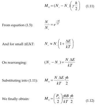
1.8 Larmor Equation

For the spin ½ proton,

m

states is:

0

B

E









By applying Planck’s Law to equation (1.6), we obtain:

0

B

hv







thus, allowing us to determine a value for the precessional frequency of the

protons using the most fundamental equation in MRI physics – the Larmor

Equation:

0

B







1.9 Net Magnetisation Vector

Although individual spins obey the laws of quantum mechanics, the average

behaviour of a group of spins (called spin packets) experiencing the same

magnetic field strength, is best described using classical mechanics. Hence, the

vector sum of the magnetisation vectors from all spin packets is represented by

Page | 10

















2

)

(





N

N

M

From equation (1.5): kT

E

e

N

N







And for small E/kT:













_





kT

E

N

N

1

kT

E

N

N

N



)





(

Substituting into (1.11):

2





kT

E

N

M





We finally obtain:

2

2









kT

B

P

M















Where Pd represents the density of protons per unit volume (Pd/2 = N-). Y

Z

B0

M0

X

Page | 11

The signal in MRI comes predominantly from M0 and its magnitude is

dependent on a number of factors, which include the magnitude of B0, the

proton density of the tissue, and the proton’s magnetic moment component

(ħ/2).

1.10 The Main Magnetic Field

Magnetic resonance imaging involves the interaction of three types of magnetic

field: the main (static) magnetic field, an oscillating radio frequency (RF) field,

and gradient magnetic fields. The primary job of the main magnetic field in

MRI is to align the spins to form the net magnetisation vector. This is achieved

using superconducting magnets as they provide a range of desirable attributes

including field strengths in the Tesla range that have excellent homogeniety

and temporal stability.

1.10.1 Superconducting Magnets

Superconducting magnets are a form of electromagnet and consist of a solenoid

(a coil of superconducting multifilament wire made of niobium-titanium alloy

embedded as fine filaments in a copper matrix). The solenoid is cryogenically

cooled to a very low temperature of around 4.2K using liquid helium. This

reduces the resistance in the wires to zero, permitting the very strong electrical

0 2 2

0

4

kT

B

P

Page | 12

currents required to create high magnetic fields to be passed through the wires

without generating significant heat. A superconducting magnetic field stores a

substantial amount of energy (Es), which can be calculated using:

2

2

1

LI

Es



Where L is the inductance of the coil windings and I is the current flowing

through them. So for a 1.5T magnet with 150 Henrys of inductance and 200

amperes of current, the stored energy would equate to 3.6MJ.

1.11 The Radio Frequency Field

In equilibrium, the net magnetisation vector aligns with the main magnetic field

along the z-axis. M0 is several magnitudes smaller than B0 (T v 1.5T). In

addition to this, M0 is not an oscillating function, and hence cannot be detected

by a receiver coil. To resolve this issue, a radio frequency (RF) pulse (B1) is

applied in a plane perpendicular to B0 (Figure 1.4).

Figure 1.4 An RF pulse is applied in a plane perpendicular to B0

Y Z

X B0

Mxy

Page | 13

1.12 Resonance

If the precessional frequency of the RF pulse matches that of the Larmor

frequency of the protons then energy is added to the system and resonance can

occur.During resonance, spins are encouraged to align with the B1field. This

phase coherence results in the formation of a net transverse magnetisation

vector in the x–y plane (Mxy) (Figure 1.4) that precesses simultaneously about B0

and B1 in a process known as nutation.

1.12.1 Rotating Frame of Reference

The concept of nutation is simplified in MRI physics by considering a rotating

frame of reference (rotating at the Larmor frequency about the z-axis). In a

rotating frame, spins rotating at the Larmor frequency appear stationary whilst

those rotating at higher or lower frequencies are seen to gain or lose phase in

comparison.

Figure 1.5 Using a rotating frame of reference simplifies the concept of flipping.

Y’

B0

M0

B1

X’

Page | 14

An observer within the rotating frame of reference will witness a simple arc

motion as the magnetisation vector is flipped from the z-axis into the x–y plane

(Figure 1.5). An observer standing outside the rotating frame of reference

would witness the more complicated nutational motion of the spins.

1.12.2 Flip Angles

The angle () through which the spins are flipped from the z-axis into the

transverse plane is referred to as the flip angle. It is the choice of amplitude, and

duration (τ) of the applied field (B1) that determines the flip angle of the

magnetisation.









B

It is possible to obtain the same angle by applying a strong pulse for a short

duration of time, or by applying a weak pulse for a longer period of time. If the

entire M0 vector is flipped into the x–y plane by the RF pulse, then the pulse is

referred to as a 90 RF pulse and the angle as a 90 flip angle. At this point:

Mxy = M0.

A 180 pulse would have twice the amplitude or twice the duration of a 90

pulse. The application of a 180 RF pulse inverts the net magnetisation vector by

exciting the excess spins in the lower energy level into the upper energy level,

Page | 15

1.12.3 Partial Flip Angles

It is possible to flip the net magnetisation vector into the x–y plane by less

than 90 simply by reducing the power and/or duration of the RF pulse.

This results in the magnitude of Mxy being less than the original magnitude

of M0:



Sin

M

M



1.12.4 Free Induction Decay

Once in the x–y plane, the precessing net magnetisation induces a voltage and

current in a receiver coil which is sensitive only to magnetic fields in the

transverse plane. This induced current is the source of the signal for all MRI

imaging.

A large signal is induced and detected immediately after a 90 pulse, as all the

spins are in phase. This signal is known as the Free Induction Decay (FID)

(Figure 1.6).

Figure 1.6 Left to its own devices the FID would quickly decay away

Amplitude

Time (ms)

Page | 16

Left to its own devices, the FID would rapidly decay away to zero as described

by the Bloch Equations (Appendix A). These macroscopic equations describe

nuclear magnetisation as a function of time when T1 (1.10.8) and T2 (1.10.9)

relaxation processes (Figures 1.7 and 1.8) are present.

1.12.5 T1 Relaxation

The T1 relaxation process is also known as the longitudinal or spin-lattice

relaxation time and describes the recovery of the Mz component of the

net magnetisation vector as it returns to its equilibrium position along the

z-axis after the application of the RF pulse. To relax back into equilibrium,

the spins have to transfer the energy gained from the RF pulse to the

environment. This transfer of energy is not spontaneous and can only happen

if the spins experience an oscillating magnetic field at or near the

Larmor frequency. The rate of energy transfer depends on a molecule’s natural

motions (rotation, vibration and translation). Hydrogen, in the form of water, is

a small molecule and therefore, moves quite rapidly. Larger molecules,

such as fat molecules move more slowly. The T1 relaxation time reflects

the relationship between the natural frequency of these molecules and

the resonant or Larmor frequency. When these frequencies are similar, the

T1 recovery of M0 is rapid, when they are very different, the T1

recovery is slow. Hence different tissues exhibit different T1 recover curves

Page | 17

The equation that describes the T1 relaxation process as a function of time (t) is:

)

1

(

)

(

0

T t

z

t

M

e

M





The T1 relaxation process also governs the recovery of the net magnetisation

vector after a 180 pulse.

)

2

1

(

)

(

0

T t

z

t

M

e

M





1.12.6 T2 Decay

The phase coherence witnessed immediately after the application of the RF

pulse is short lived as the spins interact with each other. This loss of coherence

results in the decay of the transverse magnetisation and ultimately, the loss of

signal. Again, this process varies between tissue types with larger molecules,

Page | 18

such as fat, experiencing many static internal magnetic fields in the presence of

B0due to their chemical structure. The rate of decay of Mxy is governed by the

spin-spin relaxation time (T2) of each tissue (Figure 1.8). The equation that

describes T2 relaxation as a function of time is:

) 2 / (

)

0

(

xy

xy

M

e

M



Figure 1.8 The T2 relaxation curves of the myocardial tissue and the blood pool of the heart at 1.5T.

T1 and T2 are exponential processes. In general, T2 decay is five to ten times

more rapid than T1 recovery.

1.12.7 T2* Relaxation

T2* (t-two star) is a time constant that includes the additional dephasing effects

Page | 19

inhomogeneities and magnetic susceptibility. T2* therefore, describes a quicker

loss of signal than T2 and as a result, T2* is always smaller than T2:

B

T

T

2

*



1

/

2



1

/

2





/

1

The dephasing effects that are exclusive to T2* are reversible under certain

circumstances. This reversal can be exploited in MR imaging methods [9].

1.13 Image Formation

Image formation in MRI works by defining the signal intensity in an array of

pixels so that it corresponds to a three-dimensional co-ordinate system (x, y and

z) within the patient. This is a challenging process in MRI as the signal

originates from the entire object rather than a point source and is therefore, not

simply a case of collimating the receiver coils.

In a highly homogenous magnetic field such as B0, identical spins in different

locations will precess at the same frequency and as a result, the detected signal

will contain no spatial information regarding their distribution. However, by

distorting B0with gradient fields, in a precise and controlled way, protons at

different locations will precess at different resonant frequencies. This permits

the signal amplitude to be measured as a function of frequency and phase

whilst the density of protons in the tissue allows an image of spatial structure to

Page | 20

1.13.1 Gradient Magnetic Fields

Gradients fields are small perturbations that have magnitude and direction and

are represented as vectors. They are normally applied as pulses in any chosen

direction or orientation using gradient coils. These gradient fields provide MRI

with its three-dimensional capabilities. When applied in the x, y and z direction

the gradient fields are represented by the symbols Gx, Gy, and Gz respectively.

The isocentre of the magnet is the point where x, y, and z = (0, 0, 0). The

magnetic field at this point is B0 and the resonant frequency is



1.13.2 Slice Select Gradient

The strength of the gradient characterises the slope of the field as a function of

its position along the axis. For a field gradient in the z direction:

z

G

grad

B



The Larmor frequency of each spin is therefore dependent on its position along

the axis, effectively dividing the patient into 2D slices Larmor frequencies

(Figure 1.9):

z

G

z

G

B

z









(

)





(



)



(

0

)



Page | 21

The centre frequency of the RF pulse controls the location of the slice whilst the

range of frequencies in the pulse controls the width. Protons either side of the

selected slice will be resonating at higher or lower frequencies. However, the

required frequency has to be present within the RF pulse’s transmit bandwidth

for resonance to occur, thus excitation only takes place close to the isocentre.

This allows the position, orientation and thickness of the slice to be

manipulated simply by adjusting the gradient or RF waveform properties.

1.13.3 Frequency Encoding

During imaging, a frequency encoding gradient is applied perpendicular to the

slice select gradient. Once again the centre of the slice remains unaltered but the

resonant frequency of the spins reduces to the left of the central point and

increases to the right, thus creating columns of varying Larmor frequency

within the slice.

Figure 1.9 A slice select gradient is applied that effectively divides the patient into slices of varying Larmor frequencies.

0

















Page | 22

1.13.4 Phase Encoding

The application of these two gradients is still not enough to ascribe a unique

frequency to each column and row of protons. For this reason, the signal is

encoded in terms of phase in the third direction. The phase encoding gradient

induces a change in phase that is proportional to distance, effectively dividing

the columns of spins into voxels, each with varying precessional speeds (Figure

1.10). When this gradient is switched off the spins revert to their original speeds

but keep their phase encoding until either another gradient is applied or the MR

signal decays.

Gradients are applied with or after an RF pulse. They can be applied

individually or in combination to create transverse, sagittal or coronal, oblique

or double oblique slices. During imaging, spatial localisation in the phase

encoding direction requires many steps. Each step is performed with an

The selected imaging slice is divided into voxels of spins

Apply Gx Gy

Gradients

G

G

G

Apply Gz Gradient

Page | 23

incremental change in gradient amplitude so that the protons in the same row

have the same phase but the protons in the same column have different phases.

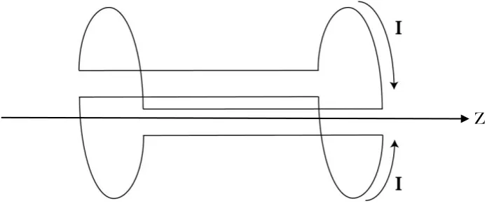
The gradient system of a modern scanner comprises of a gradient amplifier and

several gradient coils, each of which is positioned around the bore of the

magnet. The z gradient (Gz) is provided by a Maxwell pair (Figure 1.11), whilst

the x and y gradients are provided by a Golay pair

Figure 1.11 A Maxwell coil pair is the most efficient choice for producing a z-gradient (Gz).

Figure 1.12 The preferred design for a transverse gradient (Gx or Gy) is the Golay pair.

Page | 24

Modern scanners use shielded gradient coils where secondary coils are used to

cancel out undesired fields from the primary coils.

Gradient strength is a measure of the change in field strength over distance and

is directly proportional to the applied current in the coil. Gradient rise time is a

measure of the rate of change of field generated when the gradients are

switched on and off. The gradient strength divided by the rise time gives the

slew rate of the gradient coils. Slew rates refer to the speed with which the

gradients can be turned on and off. Higher gradients are desirable as they allow

thinner image slices or smaller fields of view (FOV) to be obtained without

changing any other measurement parameters.

Gradient linearity is another important factor in today’s high end scanners as

gradient non-linearity can lead to image distortion and signal loss. Thus,

manufacturers strive to restrict gradient deviations to within 5% of their desired

value.

1.13.5 Repetition Time

Typical MR experiments use a series of pulsed RF energy. The repetition time

(TR) between successive RF pulses should be long enough to allow additional

absorption during the next RF pulse and to prevent the spin system from

Page | 25

1.13.6 Echo Time

Fundamental limitations in the electronics of an MR system prevent a

measurement of the signal immediate after the application of the RF pulse.

Hence, the signal is measured after a short time period, known as the time to

echo (TE). TR and TE are intimately related to T1 and T2 respectively. However,

unlike T1 and T2, TR and TE can be adjusted and controlled by the operator.

1.13.7 Biological Parameters

T1, T2, T2* and proton density values are inherent properties of biological

tissue. Generally, T1 lengthens with increasing field strength as the energy

exchange between the spins and their surroundings is less efficient at higher

frequencies. Field strength also impacts on T2* values as higher fields have an

increased influence on intrinsic susceptibility changes in tissues.

1.14 Pulse sequences

A pulse sequence is basically an MRI software program that has the timing

parameters TR and TE embedded within it. A pulse sequence diagram

(Figure 1.11) is a timing diagram that illustrates the timings of the RF

pulses, gradients and echoes. Pulse sequences control all hardware aspects of

an MRI imaging session. Many of the advances in CMRI have resulted from

pulse sequence developments rather than hardware updates or alterations.

Pulse sequences can be used to accentuate or suppress different tissues, reduce

Page | 26

Sequences can be selected that are sensitive or insensitive to dynamic

parameters such as flow, contrast uptake or perfusion, offering exceptional

versatility.

There are two main sequence types in MRI, known as Spin Echo (SE) and

Gradient Echo (GE).

1.14.1 Spin Echo

The spin echo (SE) technique uses a 90 excitation pulse to flip the

net magnetisation vector into the x–y plane where the spins start to precess

and de-phase. A short time later (TE/2), a 180 refocusing pulse is applied

that rotates the magnetisation about the axis (Figure 1.15). Spins continue to

de-phase; however, as the magnetisation has been rotated, the spins are now

refocusing. This rotation eliminates the de-phasing effects caused by magnetic

field inhomogeneities resulting in the creation of an echo that is dependent on

T2 decay. Multiple RF refocusing pulses can be applied after the 90 RF

excitation pulse, as long as there is sufficient transverse magnetisation. This

creates a train of spin echoes.

Figure 1.15 The spin echo pulse sequence has a 90 excitation pulse followed by 180 refocusing

Page | 27

1.14.2 Spin Echo – T1 Weighted Images

Image contrast can be manipulated in SE imaging simply by varying the TR and

TE values. The selection of a long TR (e.g. 2000ms) will allow the complete (or

almost complete) recovery of the T1 curves of the different tissues. Conversely a

short TR (e.g. 300ms) will limit the time allowed for the longitudinal

magnetisation vector to fully recover and result in the incomplete T1 recovery

for some or all tissues. This results in the contrast in such images being

dependent on the T1 characteristics of the different tissue types (Table 1.1).

Thus, these images are described as being T1 weighted.

1.14.3 Spin Echo – T2 Weighted Image

Similarly, the relaxation (dephasing) rates of the transverse magnetisation

vector can provide T2 weighted images in SE if a long TR and a long TE (e.g.

80-140ms) are selected (Table 1.1). The long TR allows the complete recovery of the

longitudinal magnetisation vector and the long TE provides sufficient time for

T2 relaxation to happen. These T2 weighted images depend on the T2 relaxation

rates of the different tissues only as the application of the 180 refocusing pulse

at TE/2 refocuses the dephasing spins and cancels the dephasing effects of static

magnetic field inhomogeneities. Tissues with a long T2 provide a stronger

Page | 28 Table 1.1 The contrast in SE images is determined by the choice of TR and TE values

Spin Echo Imaging Short T2 Long T2

Short TR T1 Weighted X

Long TR Proton density T2 Weighted

1.14.4 Spin Echo – Proton Density Image

Where the operator selects a long TR and a short TE, the T1 and T2 dependence

of these images is insubstantial. For this reason, image contrast is dictated by

the density of protons in the different tissue types. Tissues with a high

Hydrogen content will appear bright whilst tissues with a low Hydrogen

content will appear dark.

1.14.5 Gradient Echo

Gradient echo (GE) pulse sequences differ from SE pulse sequences in that they

can use an excitation pulse of < 90 to produce an echo. This partial flip angle

means that at the time point TE/2, a large component of the net magnetisation

vector is lying in the z-axis. Applying a 180 pulse at this point would invert

this magnetisation (Mz) into the negative z-axis. This is not desirable as a long

TR would be required for Mzto fully recover. Alternatively, measuring the FID

would not provide the time interval essential to spatially encoding the signal.

Hence, in GE the FID is de-phased and then re-phased at a later time using a

refocusing gradient (Figure 1.16). The gradient reversal in GE sequences

Page | 29

itself and not those de-phased by magnetic field inhomogeneities. Hence, GE

image contrast is dictated by T2*.

As only one RF pulse is applied in GE, it is possible to record the signal more

quickly than in SE, resulting in a shorter TE. Partial flip angles also allow the

use of shorter TRs. Consequently, GE images are ideal for cardiac imaging as

their short TRs and reduced flip angles allow faster imaging times, significantly

reducing motion related artefacts. GE sequences are commonly referred to as

white-blood imaging, as generally blood and fat appear white in these images.

The signal weighting in a GE image depends on the TR, TE and flip angle. The

higher the flip angle, the more T1 weighted the image will be (Table 1.2). The

shorter the TE, the less T2* weighted the image will be. In addition to this, there

is an optimal combination between TR and flip angle for maximum MR signal.

The optimal angle is known as the Ernst angle (E) and is calculated from the

TR and T1 values:

Page | 30















1

exp

cos

T

TR



As the TR is always assumed to be short for a GE sequence, it has much less of

an effect on image contrast. By selecting a small flip angle the magnetisation

will be almost completely recovered, so there will be very little difference in T1

recovery curves (Table 1.2).

Table 1.2 The contrast in GE images is determined by the choice of flip angle and TE

Gradient Echo Imaging Short TE Long TE

Small flip (< 40) PD weighted T2* weighted

Larger flip (>50) T1 weighted X

1.14.6 Anatomy Scans

T1 weighted images usually have excellent contrast making it easy to

differentiate between fluids, water-based tissue and fat. For this reason, they are

commonly referred to as anatomy scans.

Page | 31

1.14.7 Pathology Scans

Fluids have the highest intensity in T2 weighted images, showing up very

brightly against the darker soft tissue. It is possible to differentiate between

normal and abnormal fluids (such as oedema) in an image as they have

different T2 relaxation rates and hence different signals. For this reason, T2

scans are considered pathology scans. Most cardiac images are acquired using a

ratio of T2 to T1 (Chapter 5).

Figure 1.14 A T2 image of the same brain highlights abnormal fluid

1.14.8 Proton Density Scans

Proton density images are dependent primarily on the concentration of mobile

hydrogen atoms within the imaging volume. The variation of proton densities

in different tissues provides the range of signal intensities and hence, image

Page | 32

1.15 Coils

In addition to the solenoid coil and gradient coils mentioned previously in this

chapter, a body coil and shim coil sets are also built in to the bore of the magnet.

1.15.1 Body Coil

The body coil surrounds the patient in the magnet bore. The main function of

this coil is to transmit the RF pulse for all scans and to receive the MRI signal

when large parts of the body are being imaged.

1.15.2 Shim Coil Sets

Shim coil sets are built into all state-of-the-art MRI systems. These coils are used

to compensate for undesirable field distortions in a passive or active manner.

Passive coils consist of shim plates (pieces of metal) that correct for field

distortions. Active coils are comprised of loops of wire that a current is passed

through to produce supplementary magnetic fields. Shim coils are essential for

cardiac imaging at 1.5T and 3.0T as they provide improved field homogeniety

across the heart. This will be discussed in Chapter 7.

Various other radio frequency coils are used in MRI to transmit energy and to

receive signals. These coils are placed on or around the region of tissue to be

scanned. They comprise of transmit receive coils, receive only coils and transmit

Page | 33

1.15.3 Surface Coils

Insulated surface coils are placed directly on top of the patient’s clothing to

ensure that the receiver is as close as possible to the MR signal. Surface coils are

commonly used in MRI as their close proximity to the patient limits the volume

from which noise is detected thus providing good SNR for superficial tissue.

1.15.4 Phased Array Coils

Phased array coils consist of an array of surface receiver coil elements with

known sensitivity profiles whose signals are combined to provide a uniform

signal intensity over a volume that is in excess of each of the smaller individual

coils (Figure 1.17). Phased array coils have a superior SNR to larger coils

covering the same area, as the design of these coils ensures that the noise from

coil to coil is largely uncorrelated.

Page | 34

This technology is ideal suited for cardiac imaging as the array can be wrapped

around the patient’s torso in a bid to obtain optimal images of the heart (Figure

1.18).

1.16 K-Space

Applying gradients in MRI changes the frequency across the patient as a

function of position effectively taking the patient from a physical space into a

frequency space. Hence, the signal we obtain is a sum of sine waves that add to

create a rapidly changing continuous voltage in our receiver coil. This complex

signal originates from every voxel in the image.

Page | 35

The signal is digitised by sampling the voltage at each point across the

echo using an analogue to digital converter (ADC). This allows the amplitude

and phase of the signal to be determined as a function of time. Each of

these points is represented by a complex number that includes a real

and `imaginary part. Rather than directly expressing position, the points

indicate the amount of spatial encoding that has taken place at that point,

with each point being identified by its value and location, which are equivalent

to the amplitude and the frequency of a sinusoid respectively.

In conventional imaging, each excitation pulse provides a single echo that

is sampled to fill a single line in k-space (Figure 1.19), with the number

of samples acquired across the echo in the x direction determining the number

of pixels in the x direction. The number of echoes sampled determines

the number of lines in the y direction, which in turn determines the number of

Figure 1.19 The signal is digitised by sampling the voltage across the echo. Each echo fills a single line in the

k-space array.

Ky

Page | 36

pixels in the y direction. Hence, filling k-space conventionally is a time

consuming process as an image with 128 pixels in the y direction would require

128 echoes each with a different phase encoding step.

It would be impossible to create an image before the gradient fields are

applied as the uniform precession of all the spins would simply create a

uniform sine wave that would superimpose as one dot in K-space. The

effective position in k-space is determined by the gradient amplitude and

duration as well as the gyromagnetic ratio.

Applying a gradient to de-phase the spins creates a temporary shift in

frequency across the sample, making the phases of the protons change as a

function of position. The spins at the centre of k-space effectively do not

experience a gradient and therefore, they do not experience a frequency shift

(



)

Page | 37 Figure 1.20 Each point in k-space is represented by a complex number that contains a real and an

imaginary part and represents the spatial encoding that has taken place at that point.

As the middle point of k-space does not experience a gradient, every proton is

in phase, providing a very strong constant signal across the image space. When

a mathematical operation [known as a Fourier transform (FT)] is performed on

the k-space array to produce the final image, this one point in k-space creates a

sheet of uniform intensity that determines the intensity of every pixel in the

image. The next point along the x-axis in k-space creates a second sheet of

intensity that has an oscillation along the x-axis but is constant in y. This

additional sheet is added to the first sheet to increasing the intensity across the

whole image, improving the spatial resolution.

The centre of k-space provides the image with contrast and the edges of k-space

provide the image with high frequency definition. Frequency is proportional to

Increasing Phase Encoding

Increasing Phase Encoding

Ky

Variation in Amplitude

Page | 38

distance from the centre of k-space. Removing high frequency data would

result in a blurred image with normal contrast.

The desired spatial resolution of the final image (Figure 1.21) is specified by

selecting the field of view (FOV) and the number of phase and frequency

encoding steps. This in turn determines the extent of the k-space array. The

more tightly packed k-space is, the larger the field of view (FOV). Conversely, if

the echo is loosely sampled a small field of view is obtained; however the pixel

size, contrast and resolution are the same.

1.17 SAR limitation

The specific absorption rate (SAR) is a measure of the rate at which energy is

absorbed by tissue when exposed to a radiofrequency electromagnetic field.

More precisely, it is a measure of the energy deposited by a radiofrequency

field in a given mass of tissue. The SAR is limited by the Medicines and

Healthcare Regulatory Agency (MHRA) guidelines [10], which state that the

FT

Page | 39

SAR must not exceed 10 W/kg of tissue for the head and trunk or 20 W/kg for

the limbs over any 6-minute period. The SAR value is affected by many

parameters such as the flip angle, amplitude of the RF pulse, selected protocol

parameters, the subject’s weight and region of exposure, and the

radiofrequency coil. To prevent limits being exceeded, the scanner will slow

imaging or suggest that a parameter is reduced, such as increasing the TR or

reducing the number of slices to be acquired.

1.18 Cardiac Magnetic Resonance Imaging

Initially, CMRI failed to gain widespread acceptance due to the challenges

associated with imaging the beating heart using a complicated technique that is

inherently sensitive to patient/organ motion. Despite this, CMRI remained an

area of intense interest within the cardiac community due to its unique

potential to provide an accurate, and reproducible, full cardiac assessment of

morphology and function, perfusion and viability, valvular disease and

coronary artery stenosis, all within a single imaging session. The sustained

development of CMRI hardware and software techniques discussed in

Chapter 3 of this thesis have resulted in a paradigm shift in CMRI’s clinical

potential, allowing it to fulfil its promise beyond the limitations of other well

Page | 40

1.19 Other Techniques and their Limitations

Although cardiac magnetic resonance imaging is now well-established and has

growing popularity within the radiology and cardiology communities, other

imaging modalities are presently utilised more frequently in clinical practice.

1.19.1 SPECT and PET

Single photon emission computed tomography (SPECT) and positron emission

computed tomography (PET) are imaging techniques that work on the same

basic principles. Patients are injected intravenously with a labelled

radioisotope, which travels through the coronary arteries to the myocardium

where it is absorbed. The decay rate of the isotope is then measured using either

a gamma camera or PET scanner, providing a functional picture of the blood

supply to the myocardium.

Figure 1.22 A series of SPECT images in three planes showing the uptake of a radioisotope in the heart

Page | 41

Single Photon Emitted Computed Tomography has become the most popular

imaging technique for the diagnostic work-up of patients with coronary artery

disease. Conversely, cardiac PET imaging initially failed to become widely

established in the United Kingdom because of its requirement for isotopes from

restricted sites with a cyclotron. However, this situation is now changing as the

required isotopes become more available.

In comparison to CMRI, SPECT and PET are immediately limited by their use

of ionising radiation. A further limitation is the difficulty in assigning cardiac

wall boundaries when coronary arteries are narrowed or occluded due to the

reduced blood flow and hence reduced isotope count in the area fed by the

diseased vessel (Figure 1.22).

1.19.2 Computed Tomography

Computed tomography (CT) is an imaging modality that is known to

provide accurate and reproducible images [11, 12] of the heart and coronary

arteries (Figure 1.23). It does this using a fan-shaped beam of x-rays that pass

through the patient to reach detectors. Subsequently, the radiation exposure

to the patient is non-trivial. This naturally restricts the use of CT for

longitudinal studies designed to chart the progression of cardiac disease-related

Page | 42

A further restriction of CT is that images can only be obtained in sagittal

or coronal planes.

1.19.3 Echocardiography

Echocardiography (echo) is the modality of choice for the detection of

heart-wall motion abnormalities that are often the earliest manifestations of coronary

blood flow restrictions. Echo is a non-ionising technique, which uses a

transducer to create a beam of very high frequency sound (ultrasound) waves

that are transmitted into the patient and reflected back. The shape, size, density

and motion of all objects lying in the path of the beam are then reconstructed on

a screen as an image (Figure 1.24).