CONTRACTIVE MARKOV SYSTEMS
Ivan Werner
A Thesis Submitted for the Degree of PhD
at the
University of St Andrews
2004
Full metadata for this item is available in
St Andrews Research Repository
at:
http://research-repository.st-andrews.ac.uk/
Please use this identifier to cite or link to this item:
http://hdl.handle.net/10023/15173
CONTRACTIVE MARKOV SYSTEMS
By
Ivan Werner
SUBMITTED IN PARTIAL FULFILLMENT OF THE REQUIREMENTS FOR THE DEGREE OF
DOCTOR OF PHILOSOPHY AT
UNIVERSITY OF ST ANDREWS SCOTLAND
NOVEMBER 18, 2004
© Copyright by Ivan Werner, 2004
ProQuest Number: 10166158
All rights reserved
INFORMATION TO ALL USERS
The q u ality of this reprod u ctio n is d e p e n d e n t upon the qu ality of the copy subm itted.
In the unlikely e v e n t that the a u th o r did not send a c o m p le te m anuscript and there are missing pages, these will be note d . Also, if m aterial had to be rem oved,
a n o te will in d ica te the deletion.
uest.
ProQuest 10166158
Published by ProQuest LLC(2017). C op yrig ht of the Dissertation is held by the Author.
All rights reserved.
This work is protected against unauthorized copying under Title 17, United States C o d e M icroform Edition © ProQuest LLC.
ProQuest LLC.
789 East Eisenhower Parkway P.O. Box 1346
UNIVERSITY OF ST ANDREWS SCHOOL OF MATHEMATICS AND STATISTICS
(i) I, Ivan Werner, hereby certify that this thesis, which is approximately 25000 words in length, has been written by me, that it is the record of work carried out by me and that it has not been submitted in any previous application for a higher degree.
(ii) I was admitted as a research student in February 2003 and as a candidate for the degree of Doctor o f Philosophy in February 2003; the higher study for which this is a record was carried out in the University of St Andrews in 2003-2004.
(iii) I hereby certify that the candidate has fulfilled the conditions of the Resolution and Regulations appropriate for the degree of Doctor of Philosophy in the University of St Andrews and that the candidate is qualified to submit this thesis in application for that degree.
signature of candidate
date W J fA k signature of candidate
UNIVERSITY OF ST ANDREW S
In submitting this thesis to the University of St Andrews I understand that I am giving permission for it to be made available for use in accordance with the regulations of the University Library for the time being in force, subject to any copyright vested in the work not being affected thereby. I also understand that the title and abstract will be published, and that a copy of the work may be made and supplied to any bona fide library or research worker.
To my grandmother
Contents
A b s tr a c t viii
A ck n o w le d g e m e n ts ix
I n tr o d u ctio n 1
1 M a rk o v sy stem s 4
1.1 Main definitions... 4
1.2 Iterations of a Markov s y s t e m ... 8
2 C o n tra ctiv e M a rk o v system s 12 2.1 In trodu ction ... 12
2 .2 CMS with continuous probabilities ... 16
2.3 CMS with Dini-continuous probabilities... 21
2.4 CMS with constant probabilities... 36
3 C o d in g m ap fo r a co n tr a c tiv e M a rk o v sy stem 47 3.1 In trodu ction ... 47
3.2 Construction w.r.t. an'outer m e a s u re ... 48 3.3 Definition w.r.t. a generalized Markov measure... 55
4 A p p lica tio n s o f th e co d in g m ap 62 4.1 Main Lemma for the generalized Markov s h i f t ... 62 4.2 What is the image of the generalized Markov measure under the coding
m a p ? ... 67 4.3 K.-S. entropy of the generalized Markov s h ift... 6 8
5 E m p iricaln ess o f th e invariant m easu re 71 5.1 In trodu ction... 71 5.2 Ergodic theorem for contractive Markov chains... 73
B ib lio g ra p h y 85
I MUST SAY TO YOU YOUNG PEOPLE
" Do n’t f o l l o w w h a t s e n i o r m a t h e m a t i c i a n s s a y t o y o u
IF YO U , YOURSELF, ARE NOT FULLY C O N V IN C E D ,"...
Abstract
We introduce a theory of contractive Markov systems ( CMS) which provides a unifying framework in so-called "fractal" geometry. It extends the known theory of iterated
function systems (IFS) with place dependent probabilities [1][8] in a way that it also
covers graph directed constructions of "fractal" sets [18]. Such systems naturally extend finite Markov chains and inherit some of their properties.
In Chapter 1, we consider iterations of a Markov system and show that they preserve the essential structure of it.
In Chapter 2, we show that the Markov operator defined by such a system has a unique invariant probability measure in the irreducible case and an attractive
prob-\
ability measure in the aperiodic case if the restrictions of the probability functions on their vertex sets are Dini-continuous and bounded away from zero, and the sys tem satisfies a condition of a contractiveness on average. This generalizes a result from [1]. Furthermore, we show that the rate of convergence to the stationary state is exponential in the aperiodic case with constant probabilities and a compact state space.
In Chapter 3, we construct a coding map for a contractive Markov system.
Acknowledgements
I would like to thank: EPSRC and School of Mathematics and Statistics of University of St Andrews for providing me with a scholarship and excellent working conditions in St Andrews, Professor K. J. Falconer and Professor A. Manning for a constructive criticism and various corrections to the thesis, my supervisor Lars Olsen for his interest in my work, his support and many fruitful discussions, Orjan Stenflo for informing me about the theory of Dependence with Complete Connections, Barry Ridge for proofreading the manuscript.
St Andrews November 22, 2004
Introduction
The study of Markov processes on metric spaces associated with a random iteration of maps has a long history which can be traced back to a paper of Onicescu and Mihoc [19]. The reader is referred to Kaijser [14], Barnsley et al. [1] and Stenflo [2 1] for historical reviews.
Our work can be seen as a continuation of works of Barnsley et al. [1] and Elton [8], which were motivated by computer modelling of "fractal" measures. This addresses a heuristic question "What is the most general randomly driven finite mechanical struc ture on a metric space which determines a Markov operator with a unique invariant Borel probability measure?".
If the metric space is finite, then one would immediately think about a directed graph with probability weights which determines a stochastic matrix - the only possible Markov operator in this case. A good candidate for such a mechanical structure handleable by a computer in a general case is a finite family o f Lipschitz maps (iue)e<= e
on the metric space with some probability functions (pe)e^E (i.e. Pe{x ) > 0 for every e G E and Y2eeEPe(x ) ~ ^ f° r x )- The Markov operator which arises from it has
2
the following form
U f := £ > . / o we for all Borel measurable functions / . eeB
Obviously, for any Borel subset B , U1b(x) defines a transition probability from the point x into the set B. Such systems have been employed for modelling different Markov processes long before (see the literature above) and were rediscovered by Hutchinson [12] (though he considered only constant probability functions) for con structions of so-called self-similar or "fractal" sets and measures supported by them. Such systems in a general setting were studied by Barnsley et al. [1] and Elton [8]. However, as we will see further (Remarks 2.1.1), their setting does not extend the case of a finite metric space, which is already very well understood. Related to the con structions of "fractal" sets, Mauldin and Williams [18] introduced a finite mechanical structure which generalizes that used by Hutchinson and extends what is known on finite metric spaces. It is called a graph-directed construction.
We introduce a theory of systems which unifies those studied by Barnsley et al. and Elton with the graph-directed constructions. •
The theory does not claim to provide the most general model concerning its prob abilistic phenomenon, since there is a general theory o f "dependence with complete connections" [13] which aims at that. However, as far as the author is aware, none of the probabilistic results presented here are covered by the existing theory.
Notation
3
(.K , d) is a metric space. All the following spaces of functions on K are real. L ip(K ) denotes the space of all Lipschitz functions, C c (K ) denotes the space of all continuous functions with compact support, C b (K ) denotes the space of all bounded continuous functions, C (K ) denotes the space of all continuous functions, C °(K ) denotes the space of all bounded Borel measurable functions. For a map u defined on K and Q C
K , u \q denotes the restriction of uon Q. For / € C b ( K ) , ||/ || is the supremum norm
of / , and j|/||<3 denotes the supremum norm of J \q for Q C K . P ( K ) denotes the set
Chapter 1
Markov systems
1.1
Main definitions
Let K i , K
2
) •••) K n be a partition of a metric space K into non-empty Borel subsets(we do not exclude the case N = 1). Furthermore, for each i E {1 ,2 ,..., N }, let
wn, wi2, ..., wiL. : Ki — > K
be a family of Borel measurable maps such that for each j E {1 ,2 ,..., L i] there exists n E {1 ,2 ,..., IV} such that (K i) C K n (Fig. 1). Finally, for each %E {1 ,2 ,..., N }, let
Pn,Pi
2
, PiLi : Ki — » M+ , ■be a family of positive Borel measurable probability functions (associated with the maps), i.e. ptj > 0 for all j and Y^jLiPij(x ) — 1 f° r all x E IQ. ■
CHAPTER 1. M A R K O V SYSTEMS 5
K
2
N = 3Fig. 1
Remark 1.1.1. (i ) Case N — 1 covers the framework from [lj and [8].
(u ) In the following, all probability functions Pij can be seen to be extended on the whole space by zero, and all maps Wij can be seen to be extended on the whole space arbitrarily. These extensions are necessary for the definition of the Markov operator
U rather than for the definition of its adjoint U* (see Definition 1.1.4). This is another
way to see how the framework from [1] and [8] can be embedded into ours.
In any arrangement o f the maps, a structure of a directed (multi)graph is easily recognized.
D e fin itio n 1.1.1. We call the set V := {1 ,..., N } the set of.vertices and the subsets
K i , ..., I<n are called the vertex sets. Further, we call the set
E := {(i,7ii) : i e { 1, ...,1V}, 7^ e {1, ...,£ < }}
the set of edges and we use the following notations:
CHAPTER 1, M A R K O V SYSTEMS 6
Each edge is provided with a direction (an arrow) by marking an initial vertex through the map
i : E — > V
0» >— ♦ j .
The terminal vertex t(j, n) £ V of an edge (j, n) £ E is determined by the corre
sponding map through
^(C7)^)) ’= ^ ^ C^i)
We call the quadruple G (V, E ,i ,t ) cldirected (multi)graph or digraph. A sequence
(finite or infinite) (..., e_i, eo, e i , ...) of edges which corresponds to a walk along the arrows of the digraph (i.e. t(ejt) = i{ek+1)) is called a path.
D e fin itio n 1.1.2. We call the family M \= (ifye), weipe) e(_E a Markov system, and we call the family without probabilities, (ATi(e), we) eg£;) a topological Markov system. D e fin itio n 1.1.3. A Markov system is called irreducible iff its directed graph is irreducible, i.e. there is a path from any vertex to any other. An irreducible Markov system is said to have a period d iff its directed graph has a period d, i.e. the set of vertices can be partitioned into d non-empty subsets f2i, ^2,..., such that
i(e) £ Pli =r* t{e) £ f^i+i mod d
for all e £ E and d is the largest with such property. An irreducible Markov system with period 1 is called aperiodic.
D e fin itio n 1.1.4. We define the Markov operator on £ ° ( K ) associated with the Markov system by
u f .= Y , p > f o w ° for a» / e C° ( K )
C H A P T E R 1. M A R K O V SYSTEMS 7
and its adjoint operator on P (K ) by
U *v{f) :=
J
U (f)d u for all / £ £ ° (K ) and v £ P {K ).D e fin itio n 1.1.5. We say a probability measure (i is an invariant probability measure of the Markov system iff it is a stationary initial distribution of the associated Markov process, i.e.
t / V = fa.
As in the case of a finite Markov chain, it is very useful to represent a Markov chain associated with a Markov system as a sequence of random variables defined on the product space of infinitely many copies of E.
D e fin itio n 1.1.6. Set
S := E z := {(•••» cf—i, o 'o ,c r i,...):c r i£ E , i £ Zi} and
£ + := E N := { { a u cr2, ...) : <r, £ E t i £ N } .
We call E+ the future of E. Consider II and E + provided with the product topology. Further, set
•' ^ Y . o"m = eJTl)o'7n-\-\ — ...,crn — for all integers m Y: ci and
i[ex, ..., en]+ := { a £ £ + : cri — e1} cr2 = e2, ..., an = en} for all n £ N.
W e call m[em, ..., en] and i [ e i , ..., en]+ thin cylinder sets. Now, for any x £ K and x[ei, .. ., e n]+ C E + , define
CHAPTER 1. M A R K O V SYSTEMS 8
Then Px extends uniquely to a Borel probability measure on E+ . Finally, for any
x £ K and k £ N, set
Zk(a) := wffk o u;(Tfc_ 1 o ... o u;CTl(cc) for all a £ E + .
It is easy to check that the sequence of random variables (Z k)kGN with respect to the measure Px represent the Markov process, associated with the CMS, with the initial distribution 5X. Moreover, obviously
Ukf { x ) =
J
f o ZkdPx for all x £ I < J £ CB{I<) and k £ N.1.2
Iterations of a Markov system
In contrast to the trivial case of finite Markov chains, here can be considered the following iterations of a Markov system.
D e fin itio n 1.2.1. Let M := ( K ( i V i j )jeJ. , {pij)jej^J ^ be a Markov system. Set
:= I<i, := Wij, pVj := Pij for all i £ 7° / , j G J° J and M ° := M .
Let the n-th iteration of M. be defined by a Markov system
M
• := (jq>,
CHAPTER 1. M A R K O V SYSTEMS 9
That can be done by the following algorithm:
1. Order the set of edges E n := { ( i j ) : i E I nJ G J f } arbitrarily, say
E n = { e u ...,e k} , k e N.
2. For each s = 1 , k, construct recursively a set Hfc(s) C K by setting
^o(s) := wCs ( / ,Q(es)) and
,(s) : = S m_ i ( s ) U A m(s), where
w e m » i f ^ m - l ( ' S ) C\ W Cm ( l f j ( e m ) ) 7^
0 , else for all m = l , ..., k.
3. Set
{/>Q*+ 1|j 6 / n+1} : = { 3 * ( l ) , . . . , 3 * ( f c ) }
by an arbitrary counting (without distinguishing the same elements in the right set). Finally, we define on each vertex set K™+1, i € I n+1, the family of maps and prob ability functions. For each i <E I n+1, there exists a unique index i G I n such that
R n+l c R U' Define
lEM
1
:= w?.and
p nM : = p ?
Kn
+1
for all j € J?CHAPTER 1. M A R K O V SYSTEMS 10
E x a m p le 1.2.1. The Fig. 2 shows the 1-st iteration of the Markov system from Fig.
1
. 'P r o p o s it io n 1.2.1. A measure is invariant w.r.t. a Markov system iff it is invariant
w. r. t. one of its iterations.
Remark 1.2.1. Trivially in the case of finite Markov chains, such iterations do not
change anything in the structure. It is known that the essential structure is preserved by such iterations in a general case as well. The directed graph associated with an iteration of a Markov system is exactly that obtained from the original directed graph
is not difficult to see that the shifts of finite type defined by two directed graphes where one is obtained from the other by state-splitting are conjugate. It means, in particular, that such iterations o f an irreducible Markov system produce irreducible Markov systems with the same period. If we decide to label the edges of the directed graph of an iteration of a Markov system simply by giving them the names of the
Fig. 2
Pr o o f. Obvious by the definition o f the iterations.
□
C H A P T E R l. M A R K O V SYSTEMS 11
maps of the original Markov system to which they correspond, then each iteration produces a softc system, but not a proper one because it defines the same sub-shift space as the original directed graph. And the difference between them is only in what we consider as separate vertex sets.
L e m m a 1.2.2. Suppose (A j(e)) we,p e) e(_E is an irreducible Markov system with an
invariant probability measure p. Then p (K i) > 0 for all i = 1,..., N .
Pr o o f. Let i
0
G V such that p ( K io) > 0. Let j G V such that there is an edgeeo from io to j . Since all probability functions are positive on their vertex sets,
it follows that p (K j ) > 0. Now, let jo G V be arbitrary. Then, by the irreducibility, there is a path from io to jo in G. Therefore, we see, through a finite repetition of
f K., , Pe0dp > 0. Then, by
^ ( K j ) =
Chapter 2
Contractive Markov systems
In this chapter we assume that (K , d) is a metric space in which sets of finite diameter are relatively compact. It implies that (if, d) is a complete locally compact separable metric space.
2.1
Introduction
If we try to represent a Bernoulli process on a finite state space, say { l ,...,i V } , as a Markov process arising from a Markov system, then we find that the underlying Markov system consists of N contractive maps, each of them maps the whole space
N } on a single point, and some constant probability functions corresponding
to them. Any other Markov chain on this state space can be obtained by changing only the probability functions. It turns out that the contractiveness of the maps has deep roots.
D e fin itio n 2.1.1 (C M S ). We call a Markov system (ifi(e), we,p e) eeE contractive iff it satisfies the following condition of a contractiveness on average: there exists
CHAPTER 2. CON TRACTIVE M A R K O V SYSTEMS 13
0 < a < 1 such that
^>^pe(x)d(w e(x ),w e(y)) < a d {x ,y ) for all x ,y 6 IQ and i € {1, . . . ,1V} (2.1.1)
eeB
(it is understood here that pe’s are extended on the whole space by zero and we’s arbitrarily). We call a Markov chain with values in K contractive iff it is determined by a contractive Markov system. We call the constant a an average contracting rate of the Markov system.
D e fin itio n 2.1.2. We call a function / : (X , d) — ■» R Dini-continuous iff there is
c > 0 such that
m * < 0 0
Jo t
where
4
> is the modulus o f uniform continuity of / , i.e.<f>(t) \= sup{|/(®) - f ( y )| : d (x ,y ) < t, x , y 6 X } .
It is easily seen that the Dini-continuity is weaker than the Hinder and stronger than the uniform continuity. There is a well known characterization of the Dini-continuity, which will be useful later.
L em m a 2.1.1. Let 0 < c < 1 and b > 0. A real function f is Dini-continuous iff
OO
<f (bcn) < oo
n= 0
where f> is the modulus o f uniform continuity of / .
CHAPTER 2. CON TRACTIVE M A R K O V SYSTEMS 14
As (j) is an increasing function,
bcn
4
>(bcn+1) ( l — c) <J
6cIl+ 1
for all n 6 N U {0 }. Hence
( l - c ) f > ( W ) < / ^ * < f > ( W ) ( l - l ) .
f»=l o n=0
□
Remark 2.1.1. Elton in [8] and Barnsley et al. in [1] considered the case N = 1 with
Dini-continuous probability functions (pe)ee£ which are bounded away from zero, and Lipschitz-continuous maps (we)eeE such that the system satisfies the following condition of a contractiveness on average: there exists 0 < r\ < 1 such that
d(we( x ) ) we(y ))Pc^ < rid(cc,y) for all x ,y € K . (2.1.2)
e £ E
There is a widely spread view in the literature that demanding condition (2.1.2) rather than (2.1.1) (with N = 1) would give a weaker assumption. However, this is not quite true.
The above Elton-Barnsley setup is equivalent to that with condition (2.1.1) (with
N —
1
) in place of (2.1.2). .Pr o o f. First, observe that the condition (2.1.1) and the boundedness away from zero of the probability functions (i.e. there exists <5 > 0 such that pe > S for all e G E) imply that the maps {we)e£E are Lipschitz. Taking the logarithm of (2.1.2)
and using its concavity reveals that (2.1.1) implies (2.1.2).
CHAPTER 2. CON TRACTIVE M A R K O V SYSTEMS 15
On the other hand, by Lemma 2.6 from [1], the Elton-Barnsley setup implies that there exist ?'i < r < 1 and 0 < q < 1 such that
' y ^pe(x)d(w e(x ),w e(y ))q < rd(x, y )q for all x , y e K . (2.1.3)
e&E
By performing a remetrization d (x, y) := d(x, y )q} which preserves the Dini-continuity of the probability functions, we can reduce it, without a loss of generality, to the
condition (2.1.1). □
In [1] Barnsley et al. realized that for the proof of the attractiveness of the invariant probability measure the condition of a uniform boundedness away from zero for the probability functions can be weakened. They came up with the following condition: there exists <5 > 0 such that
2 3 P e ( % ) P e ( y ) > S
2
> 0 for all x, y 6 K . (2.1.4)e&E: d(we(x),we(y))<rd(x,y)
In fact, now conditions (2.1.4) and (2.1.3) also cover some finite Markov chains where some transition probabilities between the states can be zero, but still very few of those which are known to possess an attractive probability measure. Moreover, the condition (2.1.4) would not work for the Elton’s proof of the corresponding ergodic theorem in [8]. So, an incompleteness of their setup is obvious and there is a need for an extension of it. Contractive Markov systems provide it in a satisfactory way.
Remark 2.1.2. (i) A similar structure was discovered by Kaijser in setup of Random
Systems with Complete Connections (RSCC) in [14]. However, what he calls weakly
distance diminishing RSCC covers only aperiodic CMS’s with compact state space,
CHAPTER 2. CON TRACTIVE M A R K O V SYSTEMS 16
eventually not after one but after a number of iterations, i.e. there exist r € N and
0 < a < 1 such that
J
d(w<Tr...w<71
x ,w (Xr...w<Tly)dPx((j) < ad(xyy) for all x ,y £ K i and i 6 { 1 , . . . , AT},where Px is a probability measure which represents the Markov process starting in x (see Def. 1.1.6). However, such systems, again just as in the case o f maps, are not expected to exhibit a substantially new behavior, but a decrease of transparency of the proofs, for such systems, can be expected.
2.2
Contractive Markov systems with continuous
probabilities
Now, we are able to prove the first theorem which shows that a CMS, under rea sonable topological assumptions which allow the associated Markov operator to map continuous functions on continuous, has some nice properties.
D e fin itio n 2.2.1. We call the partition K\, ...,Kn of K open iff every K iy i = 1,..., N, is an open subset of K . O f course, it means that K must be disconnected.
T h e o r e m 2.2.1. Suppose [K p ep w e)pe) eeE is a CMS with an average contracting
rate 0 < a < 1 such that the family K i , ..., Km is an open partition of K and each pe
is continuous on K pe). Then:
(i) The sequence (^ * fc&c)fc€N Is tight fo r all x € K , i.e. fo r all e > 0; there exists a
compact subset Q C K such that U*k5x(Q ) > 1 — e for all k € N.
(Hi) The invariant probability measure p is unique iff
1 v—•v f
— 2_J Ukg (x ) —> gdp fo r all x € K and g £ Cb{K ).
n k=i J '
(iv) If the invariant probability measure is unique, then
Y j d (x , X{)dp(x) < oo fo r all Xi € Ki, i = 1 , iV.
*=1/
CHAPTER 2. CON TRACTIVE M A R K O V SYSTEMS 17
Pr o o f, (*) Fix x^ £ Ki for each i = 1 , iV. Define N
f { x ) := 7 ; l / f .(a;)d(a;, ®i) for all x £ K
2=1
and let C > 0 be such that
m axd (we®»(e),®t(c)) < C'*
e(EE
We show inductively that
» V ( * 0 <
1 — a
for all k £ N and all i = 1 , N . First, observe that for any i £ { 1 , N } N
U f ( X i ) = ' Y ^ P e ( ^ i ) f ° W e { X i ) - y y p e { X i ) l K j ( w eX i ) d ( w e X U X j )
e e E j = 1 e e E N
= y Y ] P e ( X j ) d ( w e X j , X t{e)) < y p e ( X j ) C = C.
Suppose U ^ f i x i ) < C ( 1 - afe_1) / ( l — a) for some k. Denote by ( e i , e * . ) * a path starting in X i. Then
N
Ukf ( x i ) = y P a f f x i ) . . . p ef f w ek_1. . . w e i x i ) y 2 l K j { w ek. . . w e i x i ) d ( w ek . . . w e i x h x j )
(ei,...,e&)* 3= 1
E ^ ^ Pe\ ( X i ) ' ••Pek ••-We i X i ) d (lUek . . . W e i X i , 'lUefciCj(efc) )
(ei,...,efc)*
N
+ E
E
p ei ( ® i ) .. .p efc K _ x.. . W ei X i ) d ( w ekx i(ek)) x j )j ~ 1 (e i ek)*,t(ek) = j
N
< ^ 2 y ^ K jiW e^ .-.lU e.X i) ^ Pe
1
(xi)...pek(wek_1
..,We tXi)(e i,...,e fc_ i ) * 3= 1 ek ,i(e k ) = j
X d(w ek...WeiXi,WekXj) + C
N
- a y y j h<ffwek_x...v)eix i)peffx i)...pek_1{wek_i ...weix i)
(e i,...,e fc_ i ) * j = 1
x d ('U)ek_ 1 . . . W e i X i , X j ) + C
= aUk- lf { x i ) + C < a c H — + C =
1 — a 1 — a Let p := C / ( l — a) and e > 0. Then, by the above,
P > Ukf ( x i ) = [ f o Z £ d P Xi= f y i ( 2 ? , * , ) ^
J J j=l
> ^P x. ( d (Z f\ X j) > ^ for all j = 1, i v) for all k £ N and for a lii = 1 , N. Thus
Pxl ( d { Z l ‘ , X j ) > P- for all j = 1 ,
iv)
< efor all k £ N and for all i = 1, N . Set
N
Q * := 3= 1
CHAPTER 2. CONTRACTIVE M A R K O V SYSTEMS 19
where B p/e(y) denotes the closed ball of radius p/e and center y. Then Qe is compact (note that, since Z% are measurable, all sets considered here are measurable) and
and let Un* be its adjoint operator on P ( K ). Fix x G K . By ([i), the sequence
(Un*
6
x)neN is tight also. So, it has a subsequence Unm*5x which converges weakly* toa Borel probability measure, say p. By the hypothesis of the theorem, the Markov operator U maps continuous functions to continuous functions. Therefore, its adjoint operator U* is weakly* continuous. Hence,
> 1 - e
for all k € N and i = 1,..., N. As desired.
(ii) Define an operator
u*
o
unm*5
x) ^
u*p
asm
-> oo.However, since
-i J- *j
— E
uks ( x ) - Unm9(x)<
—2lbll for all
g G CB(K ).nm tZo nm
rl,n + l
We conclude that
U*p = p,
CHAPTER 2. CON TRACTIVE M A R K O V SYSTEMS 20
(Hi) Suppose p is the unique invariant probability measure. Then, by the above,
1 , C
— Ukg (x ) —> gdp for all x G K and g G C b (K ). (2.2.1)
n &=i J '
Conversely, if (2.2.1) holds true, by Lebesgue’s Dominated Convergence Theorem, it implies that
, , n
- V U*kA ^ p for all A G P (I<).
Again, by the weak*-continuity of U*, this implies that g is the unique invariant Borel probability measure.
(iv) Fix Xi G Ki for each i = 1 , N. Let v be the Borel probability measure on I<
given by
V(A ) := £ 5Xi(A) for all A G B (K ). i=i
Define Jr := m in {/, R } for R > 0, where / is the function from (i). Then every /r
is a bounded continuous function on K by the assumption of the theorem and, as in proof of (i),
r
N
Ukf Rd u < Y , U hf { x () < N p
J i=l
for all k G N and R > 0. Therefore,
n
:fRdv < Np
f
-J
71
k= 1for all n G N and R > 0. By (in ) and Lebesgue’s Dominated Convergence Theorem, this implies that
J
fRdg < N p for all R > 0. By Levi’s Theorem, we conclude thatJ
f dp < NpCHAPTER 2. CON TRACTIVE M A R K O V SYSTEMS 21
2.3
Contractive Markov systems with Dini-
continuous probabilities
We intend to show here that Feller contractive Markov chains with probability func tions which are Dini-continuous and bounded away from zero on their vertex sets exhibit a mixing behavior which is similar to the finite Markov chains.
The next lemma is a generalization of Lemma 2.5 from [1].
Lemma 2.3.1. Suppose (I'fye), u!e,p e) e6S is a CMS with an average contracting rate
0 < a < 1 such that Pe\i<-t ^ is Dini-continuous for all e 6 E. Then, fo r every
/ 6 C c (K ), the functions ( ^ ra/|jci)neNU{o} are uniformly equicontinuous fo r all i —
PROOF. Let cj)e be the modulus of uniform continuity of p e|/ci(e) for each e 6 E.
Note that each (f)e is non-decreasing and 4>e(t) < 1 for all t. Set
t , 0 < t < 1 1 , t > 1
and
6
:= max It is clear that d> is also non-decreasing and satisfies Dini’s e&EU{0}condition.
Let / 6 L ip (K ) and ||/|| < 1. Then there is C > 2 such that
CHAPTER 2. CON TRACTIVE M A R K O V SYSTEMS 22
where L V C := m ax{L, C }. Then /?(0) = 0, and is continuous and increasing. By the Sublemma from [2], increasing 0 if necessary, we can assume that (3 is concave. Further,
ta_1
/->/ \ n t \ L v C f (f)(u) L <j)(t) . . _ / /1\
/ J ( i ) - fla t ) = —
J
— du > — a ^ i a - ! ) =' t '
Hence
/5(at) + £</>(£) < /?(£) for alH > 0.
Note that, for 0 < t < 1,
p it)
>
Cf ‘
^ - d u > C f ‘ du = Ct,Jo
«
Joand, for t > 1, /3(t) > P (l) > C > 2. Therefore,
-I / M ~ / M l < P {d (x ,y )) for all 6 AT.
As an induction hypothesis for some n E N, assume \Un~
1
f ( x ) — t/n_1/ (2/)|< fi(d (x ,y )) for all x ,y € K i, i = 1, TV. Let rc,y 6 AT; for some i 6 {1,. .. , A } . Then, since /? is increasing and concave,
Li
|u ( e t - 1/ ) (*) - y ( y ” - ‘ / ) (j/)| < y > ; ( z ) | y " -‘ / K W ) - e t -1/ K ( ! , ) ) |
i = i Li
- p v(v)\
3= 1 Li
< ^ Z P iA x)P {d {w ij{x ),u>v(y)) + Li4>(d(xty))
3= 1
< (3{ad(x, y)) + L(j)(d(x, y))
< /?(d(a?,
2
/)).
CHAPTER 2. CON TRACTIVE M A R K O V SYSTEMS 23
Since L ip (K ) D C c (K ) is a dense subset of (C c (K ), ||.||), the claim follows by an
e/3-argument. . □
We will need to know more about properties of irreducible directed graphs. The following Lemma is a generalization of Lattice Theorem (see Theorem 4.3 in [6]). Lemma 2.3.2 (Lattice Theorem). Let an irreducible directed graph with period d
be given. Then fo r every finite path (e i,...,e n) of the digraph, there exists mo > 0
such that fo r all integers m > mo there exists a closed path o f the length md which
has ( e i , ..., en) as a part and starts with e\.
P r o o f . Let A be the set of all k E N such that there exists a closed path of the length
k which has ( e i ,..., en) as a part and starts with e\. Then A is closed under addition.
Since the digraph has period d, the greatest common divisor of numbers from A is d. Therefore, the set A contains all but a finite number of of positive multiples of d (see Theorem 1.1 o f the Appendix in [6]). In other words, there exists m0 E N such that for all m > mo there exists a path of the length md which has (ei, ...,e n) as a part
and starts with e\. □
Lemma 2.3.3. Let an irreducible directed graph with the set of vertices V and period
d be given. Fix i E V and let Vi be the set of all ordered pairs of vertices (a, (3) E V x V
which are accessible from i by paths of the same length. Then there exists r E N such
that fo r each pair (a, (5) E V* i is accessible from a and (3 by paths o f the same length
less than or equal to dr.
P r o o f . Let (a, (3) E Vi. Then there exist paths sa and sp respectively from i to a
and from i to (3 of the same length, say n^p. By the Lattice Theorem, there exists
CHAPTER 2. CONTRACTIVE M A R K O V SYSTEMS 24
which starts in i and has sa as a part. Analogously, there exists mp G N such that for all integers m > mp there exists a closed path of the length md which starts in i and has sp as a part. Set rap := m ax{m a, m p) and r := max ^ p )&v.r ap. Then there exist two closed paths of the length dr which start in i and one of them has sa as a part and the other has sp as a part. Hence, there exist two paths o.f the same length
dr — nap < dr where one of them is from a to i and the other is from (3 to i. □
The next lemma is a generalization of Lemma 2.7 from [1]. It uses a well known technique of coupling, the main idea of which is to put as much mass as possible close to the diagonal of two processes, see [14] and [15] for more on that.
Lemma 2.3.4. Suppose {fKi(e),w e,pe) e(_E is an irreducible CMS with an average con
tracting rate 0 < a < 1 such that pe\i<i{e) is Dini-continuous and there exists 5 > 0
such that pe\i<i{e) > $ fo r all e G E. Then:
(i) For every f G C c ( K ) ,
lim IUnf ( x ) — Unf(y)\ = 0 fo r all x ,y G IU and i G {1 ,..., N }
71—KX>
and the convergence is uniform on bounded subsets.
(ii) If in addition the CMS is aperiodic, then fo r every f G C c ( K )
lim |Unf { x ) — Unf(y)\ = 0 fo r all x , y G K 71—KX>
and the convergence is again uniform on bounded subsets.
P r o o f . Let S C K be bounded. We can assume S D Ki ^ 0 for all i = 1 , . . . , J V .
CHAPTER 2. CONTRACTIVE M A R K O V SYSTEMS 25
exists C > 0 such that *
m a x d (w eXi(e),Xt(e)) < G
eGE
for all Xi £ S fl Ki, i = 1 Let Xi,yi £ S D Ki for each i = . Fix
i , j £ {1, Set
E* : = E + x E + = { e : = (e i, ex, §2,. .. ) | (e i, e2, •..) £ S + , (ex, §2, £ S + }
and let P* ':= PXi <S> Pyj be the product measure on E*. Thus, if we define
Z n (e) := wen o ... o wei(xi) and Z%>(e) win o ... o wSl(yj) on E*,
then Z f ^ and Z n are independent Markov processes with initial distributions respec
tively SXi and 5yj and Unf ( x i ) — E ( f o Z ^ ) for all / £ C b {K ), where the expectation means with respect to the measure P*. Let a > 0 and for each m £ N let Ga,m be the set of all e £ E* such that
Si s.t. Z % {e),Z % (e) s K h d ( z £ ( e ) , Z « ( e ) ) < a and d ( z ? ‘ ( e ),Z * (e )') > a
for all I < m. Then (G a>m)meN are disjoint. Further, for each n £ N, set
n
Ba,n ~
S* \ |J
7 7 1 = 1
CHAPTER 2. CONTRACTIVE M A R K O V SYSTEMS 26
Bm. Now, fo r / E C c (K ),
Unf ( x i) - U " f ( y j ) = E f ( Z * < ) - E f ( z % )
= E s [ i ( 3 ? ) - / ( 3 ? ) )
7 7 1 = 1
= E S [ l G „ , m ( b ( / ( z * ‘ ) l * U - B ( / ( z » ) 1 6 m ) )
7 7 1 = 1
Further, note that for n > m
E ( / (Zn)\ Bm) = ] T P^n+A Zrn)-Pen ( w ^ O ... O We„l+
1
Z%)(em+i ,...,en)
x / («)... O ... O tuem+1Z *‘ )
=
U"-mf(Z%).
Therefore,
Unf ( x i ) - U nf ( y j ) = E B [ l Go,m ( > - " 7 ( Z £ ) - ( Z % ) ) '
7 7 1 = 1 .
+ B [ l s „ „ . ( / ( ^ ‘ ) - / ( ^ ) ) ' ■
Let e > 0 and choose, by Lemma 2.3.1, a > 0 such that for all u ,v E iCz, / = 1 , N,
d (u ,v) < o; =*> |£/"/(i0 — ^ n/ M I <
6
f° r aU n € N. ThenI C T /fe ) - £ /» / ( to)| < Y , E[ l0„,me] + E [1b„,„2|!/||] < e + 2||/||P* (B a,n) .
7 7 1 = 1
CHAPTER 2. CON TRACTIVE M A R K O V SYSTEMS 27
Sublemma 2.3.5. Suppose the CMS is irreducible and
(i) i = j or
(ii) the CMS is aperiodic.
Then P* (B a,n) — * 0 as n —*■ oo fo r all a > 0 and the convergence is uniform on S.
Pr o o f. First, observe that
. e&E
iS ^P& {Yn1') [d (weZ 'nl , wex^e^ + d(weX{ ^ , a?£(e))]
< ad (Z * \ x t{en)) P C
for all n G N. Therefore, for any natural numbers n2 > ni,
E { d { Z ^ x t^
2
))\ Z ^ ) = E [ E { d { Z % , x t^ ) \ Z % t_1
)\2%\■ < o.E[d
Repeating that we are led to
E ( d ( Z Z ,x « e„
2
))\Z £ ) < Y L - + a « -" > d .Now, let s > 2 be the largest Lipschitz constant of the maps we\jf.(e), e G E. Then,
for all n G N,
d (%n >x t{en)) — ^ (^en^nLl) ^en^Ken-l)) ~b <^('tyen‘Ct(en_i)) ^(en))
< sd (^ nl_i, ^t(e„_i)) + C* P -a.e.. Repeating it we get
CHAPTER 2. CON TRACTIVE M A R K O V SYSTEMS 28
Hence
E (d(Z£> **,>,))! K< Y P*-a.e.
Set
,= } 2 i l l o g j
and let 77-2 > 7711. Then
2C A
B ( d ( Z S ,* « K 2))| S 3 ) < 1^ = ^ So, by Markov inequality,
P* (d(Z%,xKen2))> A| X £ ) < i P*-a.e..
Analogously,
P* {d(Z»i,Vt(*„2))> A| Z “ ) < P*-a.e..
Since ( ^ ) ngN and ( ) are independent processes,
\ / nGN
P* (d (Z % ,x t M ) < A and d ( Z « , y t(e„a)) < a| Z J . Z w ) > i P ‘ -a.e.. Note that the average contractiveness condition,
^
2
pe{u)d(tueu ,w ev) < ad{u,v) for all i t , € A*, i = 1, iV, eESimplies that for every w, u 6 Ki, i = 1 , N , there exists eo € E such that d(weQu , Weo1')
< ad(n, u).
CHAPTER 2. CONTRACTIVE M A R K O V SYSTEMS 29
i.e. d = 1, there also exists r G N such that there are paths of length equal to r
between any two vertices. In both these cases, it implies that
P* ( 3i s.t. Z l‘ ,Z% 6 K -1 Z ^ , Z vJ_dr) > S** P ’ -a.e.
for all n > d r . Therefore, by the Markov property,
P" s.t. Znl2, 'fl2 > S2dr P*-a.e.
for all
112
> dr + n\. Since each we\/<\(e) is Lipschitz, there exists pdr > 0 such thatmax d (wedr o ... o w eix ^ ei), w &dr o ... o lOgj^gj)) <
p*-for all Xi,yi G /<!* C\ S, i = 1, where the maximum is taken over all paths (ei, ...,edr)* and ( § i , ..., e^r)* of the directed graph.
Now, choose k so large that ak (
2
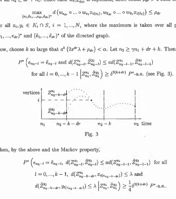
sdrX + pdr) < Let n2 > yn i + dr -f k. Then P* ^e„2_! = e„2_( and d ( 2 £ _ „ Z ® _,) < a d i Z ^ , Z ^ - , - i )for all I = 0,..., /c — 1 z u x ^ n x ) > 52(fc+rfr) P*-a.e. (see Fig. 3).
vertices
i
Z n2~ k ~ d i '
- .
ni
112
— k — dr n2 — kFig. 3
n2 time
Then, by the above and the Markov property,
P* ( en2-i = ens-ii d i Z Z ^ Z ^for all
Z = 0,..., fc — 1, d{Z^
2
_ k_ dr,Xt(en2_k_dr)) < A and [image:41.553.95.459.287.697.2]CHAPTER 2. CON TRACTIVE M A R K O V SYSTEMS 30
Observe that
d < d ( Z % _ ki wen2_k o ... o wen2_k_dr+1x t{en^ k_ dr)) + p *
+ d ( ^ e tl2_ fc O . . . O '^ e-n2_ fc_ d r+ iy t(g n2_ A;_ dr) , ^ 2 - f c )
< S^7 d ( z n ^ _ k _ d r , ® t(e„ 2 _ * _ * • ) ) P dr + s d ( y t ( e n2- k-d r)> ^ ^ - k - d r ^ j
P*-a.e.. Hence,
P* ( d ( Z * 3 * ) < ak(2sdrX + pdr)|Z£,Zg) > j<52(*!+,lr) P*-a.e..
Thus
P* ( d ( Z £ , JW) > a | z g , Z g ) < 1 - P*-a.e..
Now, choose a sequence o f natural numbers n i,ri2, ... such that n*+i > 7n* + dr + & for all t 6 N. Then, by the above and the Markov property,
/ 1 \ m—1
P* (d ( Z £ , Z g ) > a, t = 1, . . . . m j < ( 1 - -S 2<-k+dr) J for all m 6 N. Hence
/ 1 \ m_1
P* (Pa,„) < (1 - if n > n m.
Thus, P* (B^n) ^ 0 a s n - > o o and convergence is uniform on S', since 7, r, A; don’t depend on the choice of X{, yi € S, i = 1,..., iV. □
Definition 2.3.1. A measure y 6 -P(AT) is called £/ie attractive measure o f the CMS
iff
U*nv £ y for all v <E P (X ). •
CHAPTER 2. CON TRACTIVE M A R K O V SYSTEMS 31
Theorem 2.3.6. Suppose (Ki(e), w e , P e ) e e E Is an irreducible CMS such that
is an open partition of K, pe\icl{c) is Dini-continuous and there exists 5 > 0 such that
Pe|jq(e) > 5 fo r all e G E.- Then:
(i) The CMS has a unique invariant Borel probability measure p.
(ii) If in addition the CMS is aperiodic, then
Unf ( x ) —> p ( f ) fo r all x G K and f G CB{ K )
and the convergence is uniform on bounded subsets, i. e. p is an attractive probability
measure.
P r o o f , (i) Fix x { G Ki for all i = 1, Since the sequence (U*l5x.)neN is tight, (l /n S J L i ^"*l$ci)neN is a^so fight for all i — 1, ...,iV. Hence, there exists an increasing sequence of natural numbers (rik)keN such that, for each i — 1, ...,1V,
U*l&*i)ken convei’ges weakly* to a Borel probability measure, say //*, i.e.
-j nk
lim — V Ulf ( x i ) = p i ( f ) for all / € CB(K ) and %G {1 ,..., N }.
k—*oo
m-K i=i
Since, by Lemma 2.3.4 (i), for every / G C c (K ),
lim |Unf ( x i ) — Unf(jji) | = 0 for all yi G Ki and i G { 1 ,..., iV }, n—HX>
we conclude that for every / G C c { K )
-j ntc n
lim — V ' Ulf ( x ) = y > ( / ) W * ) for all x €
Since, for every x, we deal here with convergence of Radon probability measures on a locally compact metric space, it implies that
, ttfc n
lim —
V
Ulf ( x ) = y ' f t ( / ) l j f1(a:) for all a: € i f and all / e C B(I<). (2.3.1)CHAPTER 2. CONTRACTIVE M A R K O V SYSTEMS 32
Define a linear operator Q : Cb{K ) — > Cb(K ) by
n '
Q ( f ) ■= X > ( / ) 1 * for all / 6 Gb(K ). (2.3.2)
i—l
Then, by (2.3.1),
QU = Q
and therefore
Q2 = Q. (2.3.3) Now, by the definition of Hu U*Hi — Hi for all i = l,...,iV . Since the CMS is irreducible, this implies, by Lemma 1.2.2, that H i(K j) > 0 f° r hJ ~ 1»-**>N.
Now, let / G C b {K ) with / > 0. Then, by (2.3.3),
n n / N \ N
= 5 3 ^ j hu = (-Ki)
i - i i=i \ j—i J i,j=i
i.e.
N
i * ( f ) = t o W i * (k j) for a11 * = x» •••> w. j= i
Suppose there exists iq such that Hio(f) < ^ a x ^ fij(/)• Then, by the above, A*»(jf) < max P j(f ) for all* = 1, . . . , N,
l < j < N
which obviously can not be, true. Hence
M i(/) = P j{f) for all i j = 1,..., N.
Let h : = p;i. Since / G C b {K ) with / > 0 was arbitrary, we conclude that all Hu
i — 1,..., N , are equal to /i. Hence,
1 nk
lim — V C/*/(s) = n ( f ) ^ all rc G K and f 6 Cs (/^). (2.3.4) Ai—>oo ^ '
CHAPTER 2. CON TRACTIVE M A R K O V SYSTEMS 33
Suppose there exists A £ P { K ) such that
17*
A = A. Then also, nk
— U*‘ \ = A for all t e N , K i~ l
but applying Lebesgue’s Dominated Convergence Theorem to (2.3.4) implies that
Thus, A = (i, i.e. fj, is a unique invariant Borel probability measure of the CMS. (ii) Let x £ K . By Theorem 2.2.1 (i), the sequence (U*nSx)neN is tight. Therefore, there is a subsequence (U*nk5x) keN which converges weakly* to a Borel probability measure, say fi, i.e. Unkf ( x ) —> /z (/) (k —> oo) for all / £ Cb(K ). Since, by Lemma
2.3.4 (ii), |Unkf ( x ) — UUkf(y)\ —» 0 for all y £ K and for all / £ C c ( K ), it follows that Unkf { y ) —* /.i(/) for all y E I< and / £ C c ( K ) .
Let e > 0. By the tightness of (L’*n£T)n6N, there exists a compact Q C K such that
U*n5x (K \ Q ) < e for all n £ N. Hence
for all g £ C b (K ) and all n £ N. Let / £ C c { K ) . Since, by Lemma 2.3.1, the functions {Unkf\Ki) keN are equicontinuous for each i = 1, ...,1V, by Arzela-Ascoli
Theorem, there exists a subsequence, without loss of generality (Lrnfc/ ) A;eN, which converges uniformly on Q. Hence, there exists ne > 0 such that
{Z * e K \ Q } {ZfjeQ}
CHAPTER 2. CON TRACTIVE M A R K O V SYSTEMS 34
Thus, by the above,
\Unf ( x ) - K f ) \ = \Un- nH U nkf - M ) ) ( * ) \
< <\\f\\ + r i f ) ) + \Wnkf - r t f ) \ \ Q
< e( l l / l l +M/ ) + l)
for all n > n „£. Hence
Unf { x ) —*
J
fd/x for all x G K and / G C c { K ) .This also implies that
Unf ( x ) —>
J
fd/j, for all x G K and / G C b {K ),the convergence is uniform on bounded subsets by Lemma 2.3.4 (ii). By Lebesgue’s Dominated Convergence Theorem, we conclude that
U*nv (.I for all u G P ( K ) .
□
Example 2.3.1. Every irreducible finite Markov chain is a contractive Markov chain
satisfying the hypothesis of Theorem 2.3.6.
E x a m p le 2.3.2. Consider fo r simplicity R2 to be normed by ||.||i. Let K\ := [0,1] x
CHAPTER 2. CON TRACTIVE M A R K O V SYSTEMS 35
with 'probability functions
1 3 2 1
Pi := P2 := ^1/0 ) P3 •= P4 := P5 •=
l/f2-An easy calculation shows that they define a CMS with an average contracting rate
8 / 9 on K\ U K
2
U K 3} as it is shown on Fig. 4, which satisfies the hypothesis ofTheorem 2.3.6 (ii) and does not satisfy the hypothesis of Theorem 2.1 in [
1
],I<s
w2 iu4
K i
w 3
Wi
w 5 K ,
1
Fig. 4
w\ contracts K\ in the x-direction, expands it in the y-direction and maps it on K 2;
w
2
contracts K\ in the y-direction and maps it on I(3; w3
contracts K3
in thex-direction, rotates it 90° clockwise and maps it on the middle dashed rectangle in I (2;
w,i contracts I
(3
in the y-direction and maps it on the upper dashed rectangle in K\;rotates K
2
90° clockwise, contracts it and maps it on the bottom dashed rectanglein K\. Note that w$ is the only contractive map here.
[image:47.553.210.459.278.486.2]CHAPTER 2. CONTRACTIVE M A R K O V SYSTEMS 36
of finite type associated with G) provided with the metric d(a, a') :=
2
k where k is thesmallest integer with <Ji = <j[ fo r all k < i < 0. Let g be a positive, Dini-continuous
function on Ea such that
^2
9
{y) = 1 fo r all x e E GyG.T~1x
where T is the right shift map on Eg- Define, fo r every i e V,
Ki := {a € S G : t(a 0) = t}
and, fo r every e G E ,
we(a) := (..., (J—!, ctq, e), pe(a) := g ( ...,a -
1
,a0
,e ) fo r all a G K ^e).Obviously, maps {we)e€e o,re contractions. Therefore, {Ki(e),weipe) E defines a CMS
which satisfies the hypothesis of Theorem 2.3.6 and does not satisfy the hypothesis of
Theorem 2.1 in [1]. Hence, Theorem 2.3.6 (ii) covers Theorem 3.1 in [2 f] (there,
it was assumed that + n)) < 0 0 w^ere $ is ^ie modulus of uniform
continuity of lo g g w.r.t. metric d'(a,cr') — 1/ (|/c| + 1) (k is the sam,e as in the
definition of d) which is equivalent to the Dini-continuity o f g w.r.t. metric d, since
log x < x — 1 ). The invariant measure of such a CMS is called a g-measure. This
notion was introduced by M. Keane [16]. See [4], [10], [11], [22] fo r more on that.
2.4
Contractive Markov systems with constant
probabilities
For many applications, it is sufficient to consider the subsets K \ , to be compact
CHAPTER 2. CO N TRACTIVE M A R K O V SYSTEMS 37
2.3.2). For such systems, an easy proof can be given to show that their long term behaviour is analogous to the finite Markov chains by using some well known facts about stochastic matrices. We are going to present such a proof here. In addition to the results in the previous section, we show here that the rate of convergence to the stationary state is exponential in the aperiodic case with the above assumptions. So, let the subsets I<i,..., Km be compact and each probability function pe be constant and positive on K^e) and zero on the complement to K^e).
Remark 2.4.1. If N = 1 and all maps we are contractive, then we get the case
considered by Hutchinson [12].
Since with each edge e there is an associated probability weight pe, the directed.graph describes in particular a finite Markov chain with the state space V and transition probabilities
ciij := ^ 2 pe for all i , j E V,
eeEt i(e)= z, t (e )= j
provided that an initial probability distribution r := (ri, ...,77^) is given on V. Then the probability distribution on V at each following time is calculated by multiplying the distribution at the previous time as a row vector from the left with the transition matrix
A := • . ' (2.4.1)
At this point, it is appropriate to remind ourselves of some definitions and facts about finite Markov chains. G ood references for that are e.g. [5],[6].
Definition 2.4.1. (i) A finite Markov chain and its transition matrix A are called
CHAPTER 2. CON TRACTIVE M A R K O V SYSTEMS 38
(o>ij(ri))1<ij<N A n. Since aij(n) is the probability for a transition with n steps
from i to j , the irreducibility means that for alH, j € V there is always a finite path from i to j in the directed graph.
(ii) An irreducible finite Markov chain and its transition Matrix are said to have
a period d iff their directed graph has a period d, i.e. the set of vertices can be partitioned into d non-empty subsets Qi, O2, ..., Cld such that
i(e) G flj =>■ t(e ) G fA+i mod d,
for all e G E and d is the largest with such property. An irreducible finite Markov chain with period 1 is called aperiodic.
Theorem 2.4.1. Let A be an irreducible, stochastic N x N-matrix. Then there
exists a unique probability vector ro such that ?'oA = tq. Furthermore, To* > 0 fo r all
i — 1 , AT. I f the matrix is in addition aperiodic, then there exists A G [0,1) such
that
||rA n — ?’o11! < Anx(?V'o) fo r any probability vector r and n G N, (2.4.2)
where ,
and A is the positive square root of the second-largest eigenvalue of the matrix A A
where A := D ~ lA D and D := diag {roi, ...,royv} if N > 2, or A = 0 if N = 1.
Definition 2.4.2. A finite Markov chain with the property (2.4.2) is called histori
cally geometrically ergodic. y ,
Now, consider an equivalence relation on P (K ) given by
H v :<=$■ (J’(K i) = is(Ki) Vi G {1 ,..., IV}.
Let Urefl = be ^ie partition of P ( K ) which is imposed by the equivalence relation with the set of equivalence classes
P ( K )/ „ s R ■= | ( n , . . ., rN) e K N : ] [ > , = 1, r, > 0 Vi
j
. For convenience we consider R to be normed by ||.||i,N
H i r e
R-i= 1 .
Further, we define a metric L on each equivalence class M r which generates the weak*-topology on it. Set
S(I<) : = { / G C (K ) : V I < i < N V x , y G Ki |/ ( * ) - f(y)\ < d ( x , y ) }
and
L(/.i, v) := sup |fi (f) — /-'(/) | for /x, v G M r, r G R.
f e S ( i < )
Remark 2.4.2. Obviously LQu, u) > L([a, v) for /z, v G P {K ) where L is the metric
used by J. Hutchinson (see [12])
L(p.yv) = sup \ M ) - v ( f ) \ ,
L ip (f)< 1
where L ip (f) is the Lipschitz constant of / . It is well known that L generates the weak* topology on P (K ).
If ji and v are from different equivalence classes then L(p, v) is infinite.
CHAPTER 2. CONTRACTIVE M A R K O V SYSTEMS 40
Proposition 2.4.2. L is a metric on M r which generates the weak*-topology on it
fo r every r E R, and
L(/q v) < 2maxd iam (K i) fo r all g ,v E M ri r E R.
i
Proof. Let r E R. We show first that L is finite on Mr.
Let / i ,v E Mr, / G and Xi E K i VI < i < N. Then
N I M / ) - " ( / ) l <
i—1
(m, ^ r) ^ [|M(1JC. / - ljq /(z i))| + H i # , / - W ( z i ) ) | ]
i=l
N
< [diam (/Q ) g (K f) + diam (K f) v (-K*)]
Z=1
< 2 max diam (Ki). i
This shows that L (g } is) < 2maxd iam (K i).
i
By Remark 2.4.2,
L(g, u) = 0 => g = v.
The remaining metric properties are obvious. Now, we verify the equivalence
g k ^ g L (g k) g ) -> 0, for /xfcj g E Mr.
The direction “ <£=” holds true by Remark 2.4.2. For “ =>■”, let g k) g E M r with g k ^ g.
Suppose linifc^oo L (g k, g) ^ 0. Then there are e > 0 and a subsequence, without a loss
o f generality, (g k) ken such that L (g k,g ) > e V7c G N. Hence, there exists a sequence (A)fcew C S (K ) such that
CHAPTER 2. CON TRACTIVE M A R K O V SYSTEMS 41
Fix Xi E Ki for each i = 1 , N. Then the sequence (fk -fk (% i)) is equicontinuous and bounded on I<i for each 1 < i < N. By Arzela-Ascoli Theorem, it follows that there exist Qi E C(Ki) for every 1 < i < N and a subsequence, without loss of generality,
(/fc)fc€N such that ]|( f k - f k fa ) ) ~ 9i\\i<i 0 for all i. Define g := E i l i t f A /q (with
an arbitrary extension of gi on K ). Then g E C ( K ) and N
2= 1
yv
Thus
MA) - MA)I
=M
r
<
i=l
AT
2— 1 2—1
TV
2=1
+
M g ) - K g
)I
0
which is a contradiction to (2.4.3).
□
L em m a 2.4.3. (i ) For any r E R there exists s G R such that U*p G M s fo r allp G M r. Thus, the operator U* defines a map T through
T : R — >R
r i— * (U * fi(K i)i..., U *p(K ^ )), where p G M r.
(ii) For a llr E R
T (r) = rA ,
i.e. U*v G Mra fo r all v E M r, where A is the transition matrix (2.4-1).
Proof. Let p(IU) = v(IU) = : n for all i = 1,..., N. We show E/*/z(J<i) = for