1
Structural Optimisation of Random Discontinuous Fibre Composites: Part
1 - Methodology
C. C. Qian, L.T. Harper*,T.A. Turner, N.A. Warrior
Division of Materials, Mechanics and Structures, Faculty of Engineering,
University of Nottingham, NG7 2RD, United Kingdom
* Corresponding author ([email protected])
Abstract
This paper presents a finite element model to optimise the fibre architecture of components manufactured from discontinuous fibre composites. The algorithm seeks to maximise stiffness and minimise cost by determining optimum fibre distributions for local section thickness and element stiffness. The model is demonstrated by optimising the bending performance of a flat plate with three holes. Results are presented from a sensitivity study to highlight the level of compromise in stiffness optimisation caused by manufacturing constraints.
Keywords
2 1 Introduction
Discontinuous fibre architectures offer greater design freedom compared with conventional laminated composites, as the fibre orientation distribution, fibre volume fraction (Vf), and fibre length can all be locally varied in the component according to structural requirements. A number of new high volume fraction discontinuous fibre processes, such as Directed Carbon Fibre Preforming [1, 2] (DCFP) and Advanced Sheet Moulding Compounds [3] (ASMC), offer exciting opportunities for structural applications within the automotive industry. Recent developments have shown that significant gains in mechanical performance can be achieved by introducing fibre alignment [4], but the current lack of robust design tools makes it difficult to exploit the versatility of these processes, limiting these materials to ‘black metal’ design. This often results in homogeneous isotropic fibre architectures similar to those seen in lower performance moulding compounds.
Traditional optimisation routines are primarily concerned with structural issues, such as the overall mass and stiffness of the component. Topology, shape and size are the three main categories of structural optimisation and a number of methods are well established for designing with isotropic materials, but not in the context of polymer reinforced composites. The most widely used structural optimisation methods for composite materials adopt genetic algorithms, a metaheuristic type approach [5]. These are only practical for handling discrete problems and are more widely used for optimising laminated composites where local thickness is controlled by an integer number of plies. This approach is considered to be unsuitable for optimising discontinuous fibre architectures, as the number of search points increases dramatically due to the design variables (local thickness and stiffness) being continuously variable.
3 This paper presents a structural optimisation algorithm to adjust both local thickness and material stiffness for a DCFP component on an element by element basis. Stiffness optimality criteria is derived and the method of solving Lagrangian multipliers is adopted for each optimisation constraint, which include material volume and material cost. Solving Lagrangian multipliers is the classical approach to solving optimisation problems with equality constraints [9]. The local section thickness and stiffness values are updated concurrently through an iterative process, with a material cost model employed to understand the impact of increasing thickness and material stiffness during each
iteration.
Structural optimisation of meso-scale discontinuous fibre architecture composites involves a combination of continuous and discrete design variables. The local thickness can be continuously varied across the component and is independent of the fibre architecture, whereas a continuous change of fibre length or tow size is impractical and therefore can only be varied in discrete regions. A segmentation algorithm is employed to ensure that the fibre architectures generated by the structural optimisation routine are suitable for manufacture [10]. Neighbouring elements with similar material properties are merged into larger zones using a common set of material parameters (fibre length and orientation, tow size etc.), controlling the local stiffness of the zone. The size and the shape of each zone are tailored to suit the fibre deposition process, so that small areas or patches with small
dimensions are avoided. It is also rational that a critical minimum zone size exists in order to achieve a representative fibre architecture. The size of the representative volume element for achieving a homogeneous distribution of discontinuous fibres is known to be a function of fibre length and volume fraction [11, 12].
4 The modelling procedure incorporates three key areas; stiffness optimisation, material assignment and model segmentation.
2 Stiffness Optimisation
The objective of maximising the structural stiffness is equivalent to minimising the total strain energy within the structure [8]. For an isotropic, homogeneous material under a single load case subjected to a constant volume constraint, the total strain energy is minimised when the strain energy density distribution is uniform through the part [13]. In the present work, a material such as DCFP introduces an additional design variable; the effective local modulus, therefore a new stiffness optimality
criterion has been determined to optimise thickness and modulus values concurrently.
With the additional stiffness design variable, a second constraint is required to determine the limits when updating local modulus values. Restricting material cost is a sensible approach, since cost is a function of component stiffness. For example, increasing the section thickness requires a larger quantity of material to be used, whilst demanding a higher material stiffness requires an increase in fibre volume fraction or a smaller fibre tow size [14, 15]. The mechanical performance for meso-scale discontinuous fibre composites is also linked to the homogeneity of the bundle ends and the number of fibre to fibre contacts [1], therefore utilising smaller, more expensive tows yields stiffer
components.
The optimisation problem can be constructed as
min U(E, t)
subject to V(t) = V0, C(E, t) = C0
and E ≥ Emin, t ≥ tmin
(1)
5 and V0 and C0 are the target volume and cost. Emin is the lower bound of the modulus, which has been taken from the previous work on discontinuous carbon composites [1], and tmin is the lower bound for thickness, selected to prevent local buckling of the structure. The minimum thickness is influenced by the lower modulus bound, since the stiffness and strength of the component changes with thickness due to the homogeneity effects[15].
The optimisation process is performed based on the results from finite element analyses of the structure. The overall strain energy, component volume and material cost can be individually expressed as a summation of the corresponding value from each finite element in the part. The optimality criterion is derived by solving the Karush–Kuhn–Tucker (KKT) conditions of the Lagrangian expression. The Lagrangian expression from Equation (1) is
L = U + λ1(V – V0) + λ2(C – C0) + λ3(Emin - Ei) + λ4(tmin - ti) (2)
where λ1, λ2, λ3 and λ1 are the Lagrange multipliers corresponding to each constraint. The subscript i denotes the element number. The stationary of the Lagrangian leads to the following KKT conditions
𝜕𝐿 𝜕𝐸= ∑
𝜕𝑈𝑖
𝜕𝐸𝑖 + λ2∑ 𝜕𝐶𝑖
𝜕𝐸𝑖+ λ3= 0 (3)
𝜕𝐿 𝜕𝑡= ∑
𝜕𝑈𝑖
𝜕𝑡𝑖 + λ1∑
𝜕𝑉𝑖
𝜕𝑡𝑖 + λ2∑
𝜕𝐶𝑖
𝜕𝑡𝑖 + λ4= 0 (4)
If the lower bounds for modulus and thickness are inactive, then λ3 and λ4 are both equal to zero. If the number of variables is equal to the number of active constraints for an optimal design problem, then the solution yields a fully utilised design [16]. The stationary conditions in this case produce n constraint equations with n unknowns, and each can be solved independently of the Lagrangian multipliers. (i.e. each constraint equation is sufficient to determine one design variable). Therefore, Equations (3) and (4) can be rearranged as:
− ∑𝜕𝑈𝑖
𝜕𝐸𝑖 λ2∑ 𝜕𝐶𝜕𝐸𝑖 𝑖
= 1 (5) − ∑
𝜕𝑈𝑖 𝜕𝑡𝑖 λ1∑ 𝜕𝑉𝜕𝑡𝑖
𝑖 2
6 The optimality criteria can be employed based on the expressions derived in Equations (5) and (6) with an iterative scheme. The recurrence relations for modulus and thickness may be written as:
𝐸𝑖𝑘+1= (−
𝜕𝑈𝑖 𝜕𝐸𝑖 λ2𝜕𝐶𝜕𝐸𝑖 𝑖
)
1 𝑟
𝐸𝑖𝑘
(7) 𝑡𝑖𝑘+1= (
− 𝜕𝑈𝑖
𝜕𝑡𝑖 λ1𝜕𝑉𝜕𝑡𝑖 𝑖
)
1 𝑛
𝑡𝑖𝑘
(8)
where the superscript k denotes the iteration number, and r and n are the moving limit parameters to define the step size of each iteration.
The algorithms described in Equation (7) and (8) require the partial derivatives of U, V and C to be calculated for each element at each iteration. Assuming the section forces and moments applied to each element remain constant, the elemental strain energy can be written as:
𝑈𝑖 = 1
2[𝑑𝑖]𝑇[𝐾𝑖][𝑑𝑖] = 1
2[𝐹𝑖]𝑇[𝐾𝑖]−1[𝐹𝑖] (9)
where [di] and [Fi] are the element displacement and force vectors, and [Ki] is the section stiffness matrix of the ith element. Therefore, the partial derivatives of Ui are:
𝜕𝑈𝑖
𝜕𝐸𝑖 = 1 2[𝐹𝑖]𝑇
𝜕[𝐾𝑖]−1
𝜕𝐸𝑖 [𝐹𝑖] (10)
𝜕𝑈𝑖
𝜕𝑡𝑖 = 1 2[𝐹𝑖]𝑇
𝜕[𝐾𝑖]−1
𝜕𝑡𝑖 [𝐹𝑖] (11) The elemental volume is simply a function of thickness, thus
𝜕𝑉𝑖
𝜕𝐸𝑖= 0 (12)
𝜕𝑉𝑖
𝜕𝑡𝑖 = 𝐴𝑖 (13)
where Ai is the area of the ith element.
7
𝐶𝑖 = 𝛼𝐸𝑖𝐴𝑖𝑡𝑖
(14) where the factor α can be estimated by calculating the material cost for a range of DCFP laminates with known properties. The current optimisation method uses a constant cost as an equality constraint, thus the evaluation of the actual cost value is unnecessary. In future refinements to the model, an extensive database of material properties and costs would be used to provide greater fidelity. The value of α is taken as unity in the current study, which denotes the ratio of the current cost to the constraint value. Therefore;
𝜕𝐶𝑖
𝜕𝐸𝑖= 𝐴𝑖𝑡𝑖 (15)
𝜕𝐶𝑖
𝜕𝑡𝑖 = 𝐸𝑖𝐴𝑖 (16) The values of the Lagrangian multipliers λ1 and λ2 need to be correctly determined such that the overall volume and cost constraints are satisfied at every iteration, i.e.
∑ (− 𝜕𝑈𝑖
𝜕𝑡𝑖 λ1𝜕𝑉𝑖
𝜕𝑡𝑖
)
1 𝑟
𝑡𝑖𝑘 𝐴𝑖 = 𝑉0 (17) ∑ ( 𝜕𝑈𝑖
𝜕𝑡𝑖 𝜕𝑈𝜕𝐸𝑖𝑖 λ1λ2𝜕𝐶𝑖
𝜕𝐸𝑖 𝜕𝑉𝑖 𝜕𝑡𝑖 ) 1 𝑛
𝑡𝑖𝑘 𝐴𝑖 𝐸𝑖𝑘= 𝐶0 (18)
Substituting Equations (10), (11), (12), (13), (15) and (16) into Equations (17) and (18) yields a system of two non-linear equations with two unknowns λ1 and λ2, where λ1 can be determined by Equation (17), and λ2, 𝐸𝑖𝑘+1 and 𝑡𝑖𝑘+1 can subsequently be calculated from (18).
The design variables are also subjected to bound constraints, Emin and tmin. A reduced step size method is adopted here to prevent the updated value of each design variable exceeding its limit. If the output value at the current step falls below the lower bound when updating Ei and ti at the kth step (using Equations (7) and (8)), the step size parameter (r or n) is adjusted globally until the bound limits are satisfied.
3 Material Assignment
8 distribution) and converts it into a fibre areal mass distribution of constant fibre tow size and fibre length. The optimisation routine is linked to a material database containing experimental Young’s moduli for a range of DCFP plaques with various fibre architectures. The material selected for all of the studies in this paper is based on Toho Tenax 3K HTA40 at a fibre length of 30mm. For future studies of more complex components, optimum fibre parameters will be determined by a Multi-Criteria Decision Making (MCDM) strategy [17], according to design requirements such as performance, mass and cost.
For the selected carbon tow used in the current work, the material database has been analysed to form simple relationships between each fibre architecture parameter and the resultant Young’s modulus [1]. The model utilises these continuous functions to express the thickness and modulus distributions in terms of fibre volume fraction for any predetermined fibre length and tow size. The volume fraction result is then combined with the thickness result to calculate the areal mass distribution, which can be directly used to inform the robot deposition profile.
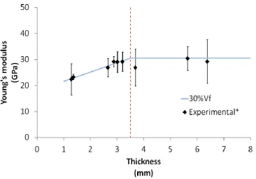
A rule of mixtures (ROM) approach is employed to summarise the relationship between Young’s modulus and fibre volume fraction for DCFP. Figure 1 shows typical data for plaques with 6K tows, chopped to a length of 57.5mm. Experimental data is presented as points, with lines representing predictions from ROM. The Young’s modulus increases linearly with increasing fibre volume fraction and the experimental points are in good agreement with the ROM predictions. Furthermore, Figure 2 illustrates that there is a tendency for the modulus to reduce for thinner specimens, which is common for discontinuous fibre architectures. It is evident that the data follows a bi-linear relationship, with a transition point occurring at 3.5mm for this particular fibre architecture. The Young’s modulus increases linearly for increasing thickness, after which a plateau is reached. This transition point depends on factors such as fibre length, volume fraction and tow size, as they all influence the level of homogeneity and departure from isotropy [12]. However in the present work, due to limited
9 It is worth noting that the current material model is only valid within certain thickness and volume fraction ranges: Very thin panels can cause buckling problems when used in real structures, and it is difficult to achieve uniform fibre distributions for very low fibre volume fractions or large tow sizes. Feasible thickness and fibre volume fraction ranges are also limited by the liquid moulding process: Preform permeability may be too low for volume fractions approaching 50%, whereas preform washing may occur if the volume fraction is too low (<15%). Whilst the thickness can be directly constrained within the stiffness optimality criterion method, the fibre volume fraction can be effectively constrained by restricting the Young’s modulus limits in Equation (1).
4 Model Segmentation Strategy
This section of the model aims to generate more realistic fibre architectures that can feasibly be produced by robotic spraying, by grouping elements of similar fibre areal mass into larger zones of uniform areal mass. The adopted approach shares many similarities with image segmentation
techniques, in particular, those based on the similarity of the pixel intensity value. The resulting zones are tailored with length scale and size control in a secondary operation.
4.1 Multi-level thresholding
Otsu’s method [18] is one of the most common thresholding methods for segmenting bi-level images. It states that the optimum threshold value should divide an image into two classes of pixels, so that the intra-class variance is minimised. A modified version [19, 20] has been used in the current paper to conduct multi-levelled thresholding.
10 Assuming K1, K2,…, KN are divided into M classes C1, C2,…, CM by M-1 thresholds, the intra-class variance can be written as:
(𝜎𝐵)2= 𝐻
𝐶1+ 𝐻𝐶2+ ⋯ + 𝐻𝐶𝑀 (19)
in which:
𝐻𝐶𝑖= 𝑆𝐶𝑖 2/𝑃
𝐶𝑖 (20)
PCi and SCi are called the zeroth-order moment and first-order moment of class Ci. Let Ka, Kb denote
the first and the last intervals within Ci:
𝑃𝐶𝑖= P(𝐾𝑎,𝐾𝑏)= ∑ 𝑝𝐾𝑛
𝑏
𝑛=𝑎
(21)
𝑆𝐶𝑖= S(𝐾𝑎,𝐾𝑏)= ∑(𝑝𝐾𝑛∙ 𝜇𝐾𝑛) 𝑏
𝑛=𝑎
(22)
where pKn is the probability that a ρA value belongs to interval Kn, and μKn is the average areal mass value of elements enclosed by Kn.
The adopted algorithm searches the optimum thresholds by calculating the intra-class variance H(Ka, Kb) for any possible class containing interval Ka to Kb (1≤a<b≤N), using Equations (20)-(22), and stores them in the following array:
[
𝐻(𝐾1,𝐾2) 𝐻(𝐾1,𝐾3) ⋯ 𝐻(𝐾1,𝐾𝑁−1) 𝐻(𝐾1,𝐾𝑁) 0 𝐻(𝐾2,𝐾3) ⋯ 𝐻(𝐾2,𝐾𝑁−1) 𝐻(𝐾2,𝐾𝑁)
⋮ ⋮ ⋮ ⋮ ⋮
0 0 ⋯ 𝐻(𝐾𝑁−2,𝐾𝑁−1) 𝐻(𝐾𝑁−2,𝐾𝑁)
11 The optimum thresholds t1, t2,…, tM-1 can be determined by calculating (σB)2 for any possible combination of H(K1,Kt1), H(Kt1+1,Kt2),…, H(KtM-1,KN) using the H array, and searches for the combination that yields a minimum value for (σB)2
.
Once all elements have been classified according to their areal mass, the model is refined into zones. A zone is defined as a group of elements that all belong to the same class and are bounded with one continuous boundary without self-intersection. The zoning process starts by randomly choosing an element as the seed. The zone expands by continuously searching and merging surrounding elements if they belong to the same class. When no further merging can be performed, a new zone will be started with a random new seed. The process continues until all the elements have been allocated a zone.
4.2 Length scale and size control
The multi-level thresholding method uses the element areal mass value as the only criteria during segmentation, and does not take into account the connectivity between elements. Therefore, model zones can result in random shapes and sizes, particularly for cases where the areal mass distribution is highly scattered. Length scale and size constraints have been enforced to remove small zones and resize any zone that contain regions narrower than can be deposited by the robotic fibre deposition head.
The minimum length scale of the zone is measured by constructing an equidistant curve from the zone boundary. The curve is formed by generating points that are perpendicular to the boundary, at a constant distance on the inside of the zone (see Figure 3).
12 boundary (solid line, Figure 3b), which encompasses elements at a constant distance r in the outward direction to form a new equidistant boundary.
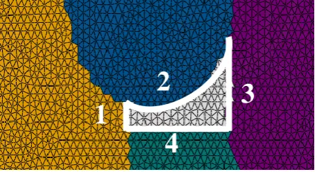
Elements removed from narrow regions are re-allocated into neighbouring zones, but steps are taken to prevent narrow regions reforming. This is demonstrated in Figure 4, where elements removed during the previous iteration (white elements) are surrounded by four other zones (coloured and numbered). The white elements are reallocated to one of the other four regions using a ‘region growth process’. Only one layer of the white elements are merged at a time and the zone is selected based on the longest boundary (in this case the row of elements bordering zone 2). Size control is performed as the last stage to reduce manufacturing complexity by minimising the number of smaller zones. It can be easily achieved by adopting a threshold value of the minimum zone size, where areas smaller than the critical size will be discarded. A subsequent merging process is required to reallocate the resultant un-zoned elements, which can be performed in the same manner as the region growth step following the length scale control.
The final outputs after segmentation and length/size control can be converted into a thickness map and a fibre areal mass map as described in Section 3,where the former can be used for the design of the RTM tool, and the latter for planning the fibre deposition program. The complete optimisation program is illustrated in Figure 5, with the initial stiffness optimisation steps on the left and the segmentation steps on the right.
5 Case Study
A 400×600mm rectangular plate (Figure 6) with three large circular holes has been chosen to
13
5.1 Finite element modelling
The CAD geometry of the plate is defined as a 3D conventional shell and exported into
ABAQUS/CAE for mesh generation and analysis. The geometry of the conventional shell represents the mid-surface of the plate, where the material properties and section thickness can be defined using the shell section definition. Quadratic elements (STRI65) are adopted for this study, but the
optimisation algorithm is capable of handling linear or non-linear conventional shell elements.
The model is subjected to a static load case using appropriate boundary conditions and is analysed in ABAQUS/Standard. The point load is applied as an equivalent pressure of 0.764MPa over a circular region of Ø10mm, to reduce the stress concentration caused by applying a concentrated force. Isotropic material properties are adopted for all material options, where composites properties are defined by the effective linear-elastic stress-strain relationship. For the steel and un-optimised
benchmark models, the corresponding shell section definition is assigned globally to the entire model, whereas for the optimised DCFP model, a *DISTRIBUTION TABLE is used to specify the shell thickness and the effective composites properties for each element. The material properties for the benchmark models have been obtained experimentally from tensile testing of straight sided samples, where the Young’s modulus and Poisson’s ratio values have been measured using digital image correlation. Table 1 summarises the material properties for the benchmark models and the optimised DCFP model. E0, t0 denote the Young’s moduli and section thicknesses respectively.
5.2 Stiffness Optimisation Results
14 level of optimisation, but the current levels have been chosen to be realistic from a manufacturing perspective.
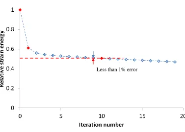
Convergence of strain energy is observed at the 10th iteration where the change in strain energy drops to less than 1% compared with the previous iteration. According to Figure 7, the total strain energy has been reduced to 48% of the un-optimised case (summarised in Table 2). It is worth noting that at this stage, since the final fibre architecture has not been determined, the variation of the effective composite density is ignored. Therefore, the constant volume constraint is effectively a constant mass constraint in this example (the mass of the two DCFP models is the same).
The thickness and modulus distributions for the optimised DCFP model are presented in Figure 8. Local changes in thickness and modulus appear in the regions where local strain energy density concentrations exist, but the patterns for each distribution in Figure 8 are different. This is because the section thickness has a greater influence on the flexural performance than the section modulus, since the bending stiffness is proportional to the modulus of the element, but proportional to the cubic of the element thickness.
It should be noted here that the thickness and modulus distributions in Figure 8 are continuously variable, which are currently impractical from a manufacturing perspective, since the fibre deposition process is difficult to control to this level of precision. This is addressed in the following section, where the zoning algorithm has been applied to group and then smooth areas of similar moduli. Continuously varying thicknesses however, can be achieved by varying the cavity height of matched tooling.
The output from this initial stiffness optimisation stage will be referred to as the ‘Initial Optimum’ in the following sections, i.e. the stiffness of the model before segmentation is implemented.
5.3 Segmentation and size control results
15 decreases, indicated by an increase in maximum deflection. For 5 levels, the maximum deflection increases by just 2% compared with the Initial Optimum presented in Figure 8. However, this error increases to 5.4% when the number of segmentation levels is reduced to 3.
Although there is a definite correlation between stiffness retention and the number of thresholding levels, it is difficult to predict the influence of different length-scale and size controls on the stiffness retention. A sensitivity analysis has been performed to determine the most appropriate segmentation strategy (thresholding levels, minimum length-scale and minimum zone size) to maximise the stiffness of the final optimised model. Models for a range of thresholding levels (3 to 6), minimum length-scales (30, 40 and 50mm) and zone sizes (2500mm2 and 6400mm2) have been studied, and the results are presented in Figure 10 in terms of the increase in strain energy compared with the Initial Optimum model.
In general, the length-scale control has the most significant influence on the subsequent change in strain energy of the model (compare to the initial optimum). The strain energy of the optimised model increases with the minimum length-scale. Increasing the number of thresholding levels also causes a further rise in strain energy, as it increases the likelihood of small, narrow zones forming. These subsequently get modified during the length-scale control, which is reflected in the associated changes in strain energy. Size control has a minor impact for all scenarios in Figure 10, and its influence becomes even less significant as the number of thresholding levels and the minimum length-scale increase. It is interesting that some scenarios are not affected by the subsequent size control at all, which is because the previous length-scale control has effectively removed zones that are smaller than the minimum size.
length-16 scale and 6400mm2 min. size) the structural stiffness is still 38.6% higher than the un-optimised case (the 4mm thick DCFP benchmark). This compromise is considered to be essential for some
components in order to produce realistic fibre architectures that are suitable for manufacture.
Results from the sensitivity analysis have shown that the length-scale control represents the biggest compromise to the stiffness when compared to the Initial Optimum. In order to minimise the effect of the segmentation process, all parameters need to be carefully selected. For example, the number of thresholding levels directly influences the number of zones, and therefore must be minimised to reduce the length and complexity of the robot program. The length-scale of the zone needs to be large enough to achieve representative material properties; to reduce variation and improve reliability, as demonstrated in [11, 12]. The minimum length-scale is also influenced by the fibre deposition cone of the chopper gun, but the selected value should be minimised to reduce the resulting compromise in stiffness. Finally, the minimum zone size is also important in terms of preform variability, as boundary effects can increase as zone size decreases.
According to Figure 10, the highest stiffness retention (92.5%) is achieved from 5 thresholding levels, using a minimum length-scale of 30mm and a minimum zone size limit of 2500mm2. Figure 11 shows the progression of the model segmentation stage. It is clear that applying length-scale and size control reduces the complexity of the zones, but as a compromise, the minimum deflection increases by 7.7% compared with the Initial Optimum model.
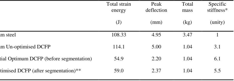
5.4 Results Summary
An overview of the bending results is presented in Table 2 for the three candidate materials. Values for the ‘optimised DCFP’ scenario are presented in two stages, before (Initial Optimum) and after segmentation. The segmentation strategy was chosen based on the results from the sensitivity study above (5 thresholding levels, minimum length-scale of 30mm and a minimum zone size limit of 2500mm2).
17 therefore the specific stiffness is 3 times higher. Following stiffness optimisation, the specific stiffness of the Initial Optimum increases to 6.1 compared with the steel plate, but this is subsequently reduced to 5.5 when the segmentation strategy is applied. This equates to a reduction in peak displacement of over 52% compared with the steel plate, for a panel that weighs less than one third.
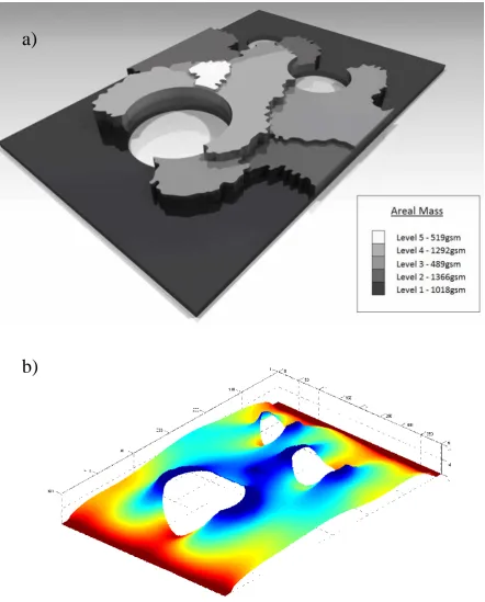
The final output from the optimisation model is presented in Figure 12, in the form of a preform areal mass map and a 3D contour of the tool surface. The areal mass map is taken from Figure 11,
following segmentation. Discrete areal masses have been shown for each layer, to facilitate robot programming. A 1018gsm base layer of fibre is sprayed over the entire surface, followed by local patches of reinforcement. The total areal mass in the central region is 4684gsm, following the deposition of the fifth and final layer. The preform is shown to be net-shape, but it is assumed that some trimming may be required to define details such as holes, in order to ensure that the target areal mass is achieved without encountering boundary effects.
The mould contour in Figure 12b represents the cavity of a matched tool, which is derived from the thickness profile in Figure 8. The thickness of the part is mirrored about the mid-plane, as assumed for the shell-thickness definition in the FE analysis.
6 Conclusions
A stiffness optimisation method has been developed to locally vary the thickness and fibre areal mass distribution for structural components manufactured from discontinuous fibre composites. This tool has been designed to overcome the challenges typically associated with using heterogeneous materials; to exploit their versatility and offer aggressive cost and weight savings over unoptimised alternatives.
18 The optimisation algorithm has been demonstrated using a flat rectangular plate with three holes. Results from this case study suggest that the current method can effectively improve the stiffness of the component without sacrificing weight-saving potential or adding additional cost over the original benchmark. A sensitivity study has shown that that the length-scale control of the segmentation process represents the biggest compromise to the stiffness when compared to the Initial Optimum. The length-scale therefore needs careful consideration to ensure that the zone size is large enough to achieve representative material properties and that the preform is fit for manufacture, but small enough to minimise the associated compromise in stiffness.
The case study presented in this paper only demonstrates the basic capability of the model; to maximise the stiffness by determining the optimum areal mass and thickness distributions. The fibre architecture (fibre length, tow size etc.) is chosen upfront and therefore the optimisation solution is specific to that one case. The second part of this paper [21] presents a material selection algorithm to determine optimum fibre architectures from the large range of experimental data available, according to additional mass and cost constraints. Multiple solutions are derived and a Multi-Criteria Decision Making strategy is adopted to rank candidate materials according to different weighting strategies. A more complex automotive case study is used to demonstrate this development.
7 References
[1] Harper, L.T., T.A. Turner, N.A. Warrior, J.S. Dahl, and C.D. Rudd, Characterisation of random carbon fibre composites from a directed fibre preforming process: Analysis of
microstructural parameters. Composites Part A: Applied Science and Manufacturing, 2006.
37(11): p. 2136-2147.
[2] LUCHOO, R., L.T. HARPER, M.D. BOND, and N.A. WARRIOR, Net shape spray
deposition for compression moulding of discontinuous fibre composites for high performance
19 [3] Feraboli, P., T. Cleveland, M. Ciccu, P. Stickler, and L. DeOto, Defect and damage analysis
of advanced discontinuous carbon/epoxy composite materials. Composites Part A: Applied
Science and Manufacturing, 2010. 41(7): p. 888-901.
[4] HARPER, L.T., T.A. TURNER, J.R.B. MARTIN, and N.A. WARRIOR, Fiber alignment in directed carbon fiber preforms - a feasibility study. Journal of Composite Materials, 2009.
43(57): p. 57-74.
[5] Jakiela, M.J., C. Chapman, J. Duda, A. Adewuya, and K. Saitou, Continuum structural topology design with genetic algorithms. Computer Methods in Applied Mechanics and
Engineering, 2000. 186(2-4): p. 339-356.
[6] Yang, R.J. and C.H. Chuang, Optimal topology design using linear programming. Computers & Structures, 1994. 52(2): p. 265-275.
[7] Svanberg, K., The method of moving asymptotes—a new method for structural optimization. International Journal for Numerical Methods in Engineering, 1987. 24(2): p. 359-373. [8] Feury, C. and M. Geradin, Optimality criteria and mathematical programming in structural
weight optimization. Computers & Structures, 1978. 8(1): p. 7-17.
[9] Lam, Y.C., D. Manickarajah, and A. Bertolini, Performance characteristics of resizing algorithms for thickness optimization of plate structures. Finite Elements in Analysis and
Design, 2000. 34(2): p. 159-174.
[10] Luchoo, R., L.T. Harper, M.D. Bond, N.A. Warrior, and A. Dodworth, Net shape spray deposition for compression moulding of discontinuous fibre composites for high performance
applications Plastics, Rubber and Composites, 2010. 39: p. 216-231.
[11] Harper, L.T., C. Qian, T.A. Turner, S. Li, and N.A. Warrior, Representative volume elements for discontinuous carbon fibre composites – part 1: Boundary conditions. Composites
Science and Technology, 2012. 72(2): p. 225-234.
[12] Harper, L.T., C. Qian, T.A. Turner, S. Li, and N.A. Warrior, Representative volume elements for discontinuous carbon fibre composites – part 2: Determining the critical size. Composites
20 [13] Venkayya, V.B., Optimality criteria: A basis for multidisciplinary design optimization.
Computational Mechanics, 1989. 5(1): p. 1-21.
[14] HARPER, L.T., Discontinuous carbon fibre composites for automotive applications, in PhD Thesis. 2006, The University of Nottingham: Nottingham.
[15] Kirupanantham, G., Characterisation of discontinuous carbon fibre preforms for automotive applications in Mechanical Engineering. 2013, University of Nottingham.
[16] Patnaik, S.N., J.D. Guptill, and L. Berke, Merits and limitations of optimality criteria method for structural optimization. International Journal for Numerical Methods in Engineering,
1995. 38(18): p. 3087-3120.
[17] Figueira, J., S. Greco, and M. Ehrgott, Multiple criteria decision analysis: State of the art surveys. Vol. 78. 2005: Springer.pp
[18] Otsu, N., A threshold selection method from gray-level histograms. Systems, Man and Cybernetics, IEEE Transactions on, 1979. 9(1): p. 62-66.
[19] Liao, P.-S., T.-S. Chen, and P.-C. Chung, A fast algorithm for multilevel thresholding. Journal of Information Science and Engineering, 2001. 17: p. 713-727.
[20] Huang, D.-Y. and C.-H. Wang, Optimal multi-level thresholding using a two-stage otsu optimization approach. Pattern Recognition Letters, 2009. 30(3): p. 275-284.
[21] Qian, C.C., L.T. Harper, T.A. Turner, and N.A. Warrior, Structural optimisation of random discontinuous fibre composites: Part 2 - case study. Composites Part A: Applied Science and
Manufacturing, 2014. Under review.
8 Tables
Table 1: Material properties for the structural optimisation model. Benchmark values for DCFP are taken from 3K 30mm fibre length at 30%Vf [15].
21
(MPa) (MPa) (MPa) (mm) (mm) (mm) Kg/m3
Steel 200000 - - 0.3 2 - - 7850
[image:21.595.68.547.248.415.2]DCFP 27060 15000 45000 0.3 4 2 6 1230
Table 2: FEA results for the benchmark model and the optimised DCFP. Total strain
energy
Peak deflection
Total mass
Specific stiffness*
(J) (mm) (kg) (unity)
2mm steel 108.33 4.95 3.47 1
4mm Un-optimised DCFP 114.1 5.00 1.04 3.1
Initial Optimum DCFP (before segmentation) 54.9 2.20 1.04 6.1
Optimised DCFP (after segmentation)** 59.0 2.37 1.04 5.5
*Values normalised to the benchmark case of steel.
**Zones created with 5-level thresholding, 30mm minimum length-scale and 2500mm2 minimum zone size.
22 Figure 1: Young's modulus vs. fibre volume fraction for 6K, 57.5mm DCFP. Em indicates the Young’s modulus of the unreinforced matrix. Experimental data includes tensile specimens of different thickness ranges as indicated with marker shape and colour intensity. Solid lines indicate the ROM relationship for constant specimen thickness. Error bars indicate the standard deviation of the experimental Young’s moduli.
Figure 2: Young's modulus vs. specimen thickness for 6K 57.5mm DCFP. Experimental data are normalised to 30%Vf using Rule of Mixture. Error bars indicate the standard deviation of each specimen type.
Figure 3: The equidistant boundary approach to control the minimum length scale of a zone. All solid lines indicate reference boundaries and all dotted lines indicate corresponding equidistant boundaries.
Singularity
[image:22.595.81.448.197.452.2] [image:22.595.76.511.548.688.2]23 Figure 4: Schematic diagram of the region growth process. The white region in the centre indicates the un-zoned elements and the coloured, numbered regions indicate the existing zones.
2
3
[image:23.595.73.302.110.234.2]24 Figure 5: Flow chart of the structural optimisation algorithm
CAD shell structure
FEA modelling – Generate conventional
shell elements
Assign element thickness (ti) & modulus (Ei)
Static isotropic analysis
Output element strain energy Ui
Total strain energy converged?
Update ti & Ei
(Stiffness optimisation) Initial Optimum (w/o zones) Material test/virtual coupon test Material database Create zones (Multilevel thresholding) Remove narrow regions (Length-scale Control)
Reallocate elements Remove small zones
25 Figure 6: Geometry of the plate. A point load is applied at the centre of the plate in the through-thickness direction, as indicated by the red circle.
Figure 7: Convergence of strain energy (normalised to un-optimised value) during stiffness optimisation process.
[image:25.595.84.462.376.646.2]26 Figure 8: Thickness (left) and modulus (right) distribution of the DCFP plate after stiffness
optimisation (Initial Optimum).
Figure 9: Examples of the preform fibre areal mass distribution of the optimised model after
segmentation with multi-level thresholding. Areal mass value for each level (high to low) is 5117gsm, 2893gsm and 1162gsm for 3-level model; and 5408gsm, 4096gsm, 3046gsm, 2183gsm and 987gsm for 5-level model.
Modulus (MPa) Thickness (mm)
Initial Optimum
Max. deflection
2.20mm
3 levels
Max. deflection
2.32mm
5 levels
Max. deflection
2.25mm
[image:26.595.89.494.425.642.2]27 Figure 10: Effect of varying the number of thresholding levels, minimum length-scale and minimum zone size on the structural stiffness of the plate. Increase in strain energy is normalised to the ‘Initial Optimum’ model.
Figure 11: Examples of the areal mass distribution after applying length-scale control and size control. (a) After 5-level thresholding (2.25mm max. deflection), (b) after 30mm length-scale control
(2.36mm max. deflection) and (c) after 2500mm2 zone size control (2.37mm max. deflection).
Zones too small for manufacture
Areal mass (gsm)
a) b) c)
[image:27.595.80.485.445.660.2]28 Figure 12: Final output from the optimisation model in the form of a) preform areal mass map and b) 3D contour for the mould tool. (Thickness scaled for clarity (in mm))