EVOLVED STARS OF LOW MASS
Robert A. Malaney
A Thesis Submitted for the Degree of PhD at the
University of St Andrews
1986
Full metadata for this item is available in St Andrews Research Repository
at:
http://research-repository.st-andrews.ac.uk/
Please use this identifier to cite or link to this item:
http://hdl.handle.net/10023/4604
This item is protected by original copyright
by
R. A. Malaney
A dissertation submitted for the degree of Doctor of Philosophy at the University of St. Andrews
I certify that Robert Anderson Malaney has spent nine terms in research work at the University Observatory, St. Andrews, that he has fulfilled the conditions of Ordinance General No. 12 and Senate Regulations under Resolution of the University Court, 1961, No.1, and that he is qualified to submit the accompanying dissertation in application for the degree of Ph.D.
Except where reference is made to others, the research described in this thesis and the composition of the thesis are my own work. No part of this work has been submitted for another degree at this or any other University. Under Ordinance General No. 12, I was admitted to the Faculty of Science of the University of st. Andrews as a research student on 1st. October 1982, to carry out an investigation on the origin of the hydrogen deficiency observed in some evolved stars. I was accepted as a candidate for the degree of Ph.D. on 1st. October 1983, under Resolution of the University Court, 1967,No. 1.
use in accordance with the regulations of the University Library for the time being in force, subject to any copyright vested in the work not being affected thereby. I also understand that the title and abstract will be published, and that a copy of the work may be made and supplied
ABSTRACT
The origin of the extreme hydrogen deficiency observed in the R Coronae Borealis (RCrB) stars remains poorly understood. A likely mechanism for producing this deficiency is one whereby the original hydrogen envelope of the star is engulfed and destroyed in its interior. One of the few RCrB stars so far analysed, U Aquarii, in fact shows emphatic evidence of such an event having indeed occurred. This evidence takes the form of the large s-process enhancements observed in
U Aquarii. Such enhancements are caused by the production of significant neutron fluxes which are directly produced by envelope engulfment giving rise to the 12 C(p,~) 13 N(ft y) + 13 C(O<,n) 16 0 sequence of nuclear reactions. In order to obtain vital information regarding the nature of the envelope mixing event from observed s-process enhancements, detailed nucl eosynthesis calculations investigating neutron production and s-process synthesis are carried out using a series of nuclear reaction networks and covering a wide range of parameter space. These calculations are mainly based on low-mass AGB and post-AGB stellar models since it is widely believed that the RCrB's are in some way related to this group of stars. It is shown how the ingestion rate of envelope material, the initial abundances and the type of mixing model used have a large influence on the neutron and s-process production.
ACKNOWLEDGEMENTS
I am indebted to supervisor, Dr. P.W.Hill, for support, guidance and help during the period of ~ studies
hls
CONTENTS
CHAPTER 1. INTRODUCTION
1.1) Stellar Neutron Synthesis
1.2) Discovery of Extremely Hydrogen Deficient Stars 1.3) Evolution of EHe and RCrB Stars
1.4) Mixing Mechanisms 1.5) Abundance Analyses 1.6) Variabili ty
1.7) Plan of Thesis
CHAPTER 2. BASIC NUCLEOSYNTHESIS THEORY
2.1) Nuclear Reactions in Stellar Interiors a) Generalities
b) Non-Resonant Reactions c) Resonant Reactions d) Neutrons
e) Beta Decay
2.2) Heavy Element Synthesis by the S-Process 2.3) Numerical Analysis of a Reaction Network
a) Numerical Solution b) Errors
c) Computations
2.4) The Reaction Networks
CHAPTER 3. NEUTRON PRODUCTION AT A HELIUM SHELL FLASH 3.1) The Helium Shell Flash
a) Details of the Flash b) Neutron Sources 3.2) Calculations
3.3) Results
a) Parameters Affecting Neutron Production b) Effect of Intershell Splitting
c) Delayed Mixing by Semiconvection
CHAPTER 4. HEAVY ELEMENT SYNTHESIS 4.1) Preliminary Calculations
4.2) Fe to Mo Enhancement Neglecting Intershell Splitting 4.3) Fe to Mo Enhancement Including Intershell Splitting
a) Total Element Enhancement
b) Individual Isotopic Enhancement 4.4) Repeated Shell Flashes
4.5) Conclusions
CHAPTER 5. COARSE DIFFERENTIAL ABUNDANCE ANALYSIS OF U AQUARII 5.1) Discovery of Sr and Y Enhancements in U Aquarii
5.2) Observations and Method of Analysis 5.3) Results
5.4) Conclusions
CHAPTER 6. THE ORIGIN OF U AQUARII 6.1) Hydrogen Deficiency
6.2) tGB and Post-AGB Comparison
6.3) Nature of the Neutron Exposure 6.4) The Helium Core Flash
6.5) FG Sagittae 6.6) Conclusions
CHAPTER 7. PHOTOMETRIC STUDY OF EXTREME HELIUM STARS 7.1) Purpose for Photometric Study of EHe Stars 7.2) Variability of BD-904395
a) Observations
CHAPTER 8. CONCLUSIONS AND FUTURE WORK
8.1) Neutron Production in Low-Mass AGB and Post-AGB Stars 8.2) Heavy Element Production
8.3) Origin of the RCrB and EHe Stars
8.4) Future Analyses of RCrB Type Spectra 8.5) Future Calculations
APPENDIX
TABLFS Table 1.1 Table 1.2
Table 2.1 Table 2.2
Table 3.1 Table 3.2 Table 3.3 Table 3.4 Table 3.5
Table 3.6
Table 3.7
Table 3.8
Table 3.9 Table 3.10
Table 4.1 Table 4.2 Table 4.3 Table 4.4 Table 4.5 Table 4.6 Tabl e 4.7 Table 4.8 Table 4.9 Table 4.10
Known EHe stars Known HCrB stars
Light particle network
Heavy element network (no branching)
Properties of 13th and 24th flashes Initial abundances
Changes of light particle abundances Summary of peak neutron fluxes
13 C/ 14 N and neutron fluxes following splitting 4 S 0
for T
b=2. x10 K
13
c
/14N and neutron fluxes following splittingS 0
for T
b=2.75x10 K
13
c
/14N and neutron fluxes following splitting for Tb=2.75x10
S oK and for low initial carbon
Different 13
c
/14N and neutron fluxes following splitting 4 SOfor Tb=2. x10 K
Initial 13 C rich region
Neutron densities arising from Iben and Henzini mixing
Initial abundances for initial heavy element calculations Heavy element preliminary enhancements
Enhancements from 2.5x10⁻⁵M mixing (no splitting)
o
Enhancements for different average flux conditions Enhancements after intershell splitting
Enhancements of the individual isotopes of table 4.5 Final enhancements for figures 4.9 to 4.20
Isotopic enhancements for figures 4.9 to 4.20 Direct repeated mixing enhancements
Table 5.2 Table 5.3 Table 5.4 Table 5.5 Table 5.6
Tabl e 6.1 a Tabl e 6.1 b Table 6.2 Table 6.3
Table 7.1 Table 7.2 Table 7.3
Table 8.1
Equivalent widths [N
F e
IN ]
op For Fe! lines Logarithmic abundances[EI/Fe] Ratios of U Aquarii relative to HD182040
Observed abundances compared to exponential exposure curve
Comparison of models of table 4.5 for d=10 Comparison of models of table 4.5 for d=30
Comparison of models for repeated shell flash calculations Observed FG Sagittae enhancements
o
BD-9 4395 photometry
o Adopted frequency solution for BD-9 4395
o
BD+1 4381 photometry
FIGURES Figure 1.1 Figure 1.2 Figure 1.3
Figure 2.1 Figure 2.2 Figure 2.3 Figure 2.4
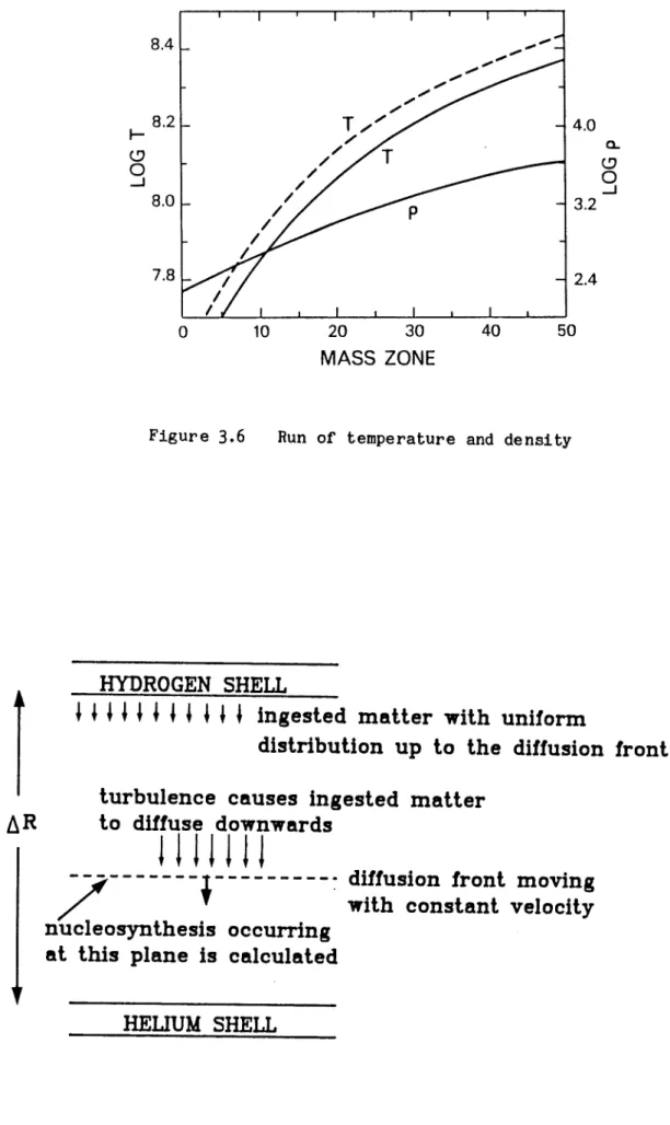
Figure 3.1 Figure 3.2 Figure 3.3 Figure 3.4 Figure 3.5 Figure 3.6 Figure 3.7 Figure 3.8
Figure 3.9 Figure 3.10
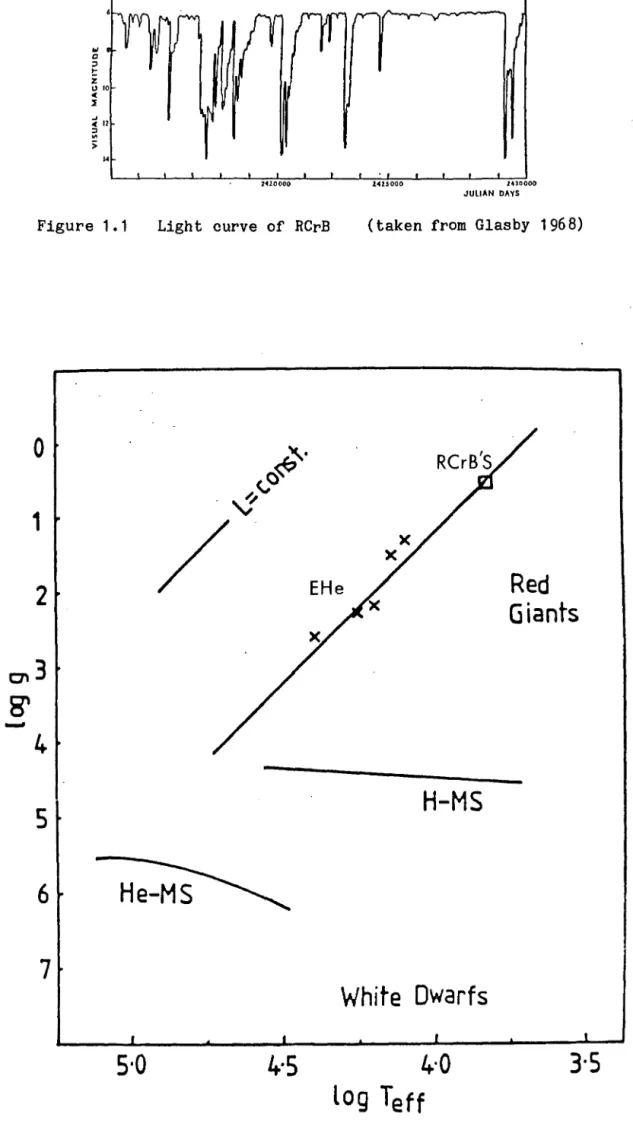
Light curve of RCrB
Evolutionary track of RCrB-EHe stars in Log g-Log Teff plane 1.45M evolutionary track o
Tunnelling effect of particle with E
<
E c 0- (E) behaviourNuclear branching diagram Fe to Mo reaction network
Basic structure of low-mass AGB star
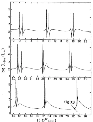
Luminosity behaviour for 7th 8th and 9th flashes
Luminosity of helium, hydrogen and total for 9th flash Structure at maximum convection extent
Schonberner evolutionary track Run of temperature and density
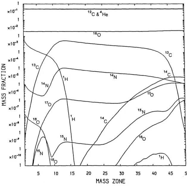
Diffusion of ingested envelope material -6
Mixing of 2.5x10 Me of envelope material into an intershell with T
b=2.4x10⁸ oK
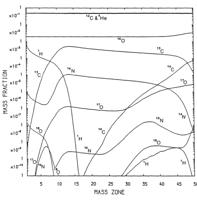
Same as figure 3.8 only showing effect of high in! tial 18 0
-6
Mixing of 2.5x10 Me of envelope material into an intershell with T
b=2.75x10⁸ oK
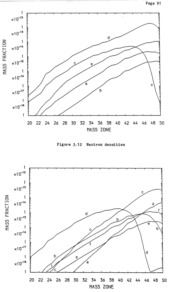
Figure 3.11 Same as figure 3.10 only neglecting absorptions on heavy nuclei Figure 3.12 Neutron densities
Figure 3.13 Figure 3.14 Figure 3.15 Figure 3.16
Figure 4.1
Neutron densities for v varied c
Final zone abundances for 10x2.5x10-7M Final zone abundances for 10X2.5x10-6M
13
c
/14N ratio as a function of mixingPath of linear flow-no branching
0 mixing 0 mixing
Figure 4.2 Heavy element enhancements Br to Zr as function of time (from model B table 4.5)
(from 2nd model table 4.4)
Figure 4.4 Late slow flux on total element enhancements Figure 4.5 Light particle reactions
Figure 4.6 Importance of unthermalised nuclei
Figure 4.7 Late ~nthesis by slow flux on individual isotopes Figure 4.8 1" as a function of shell flash
Figure 4.9a Repeated mixing for 1"=0.7, thermalised 4.9b
Figure 4.10a Repeated mixing for 1"=0.7, unthermalised 4.10b
Figure 4.11 a Repeated mixing for 1"=0.8, unthermalised 4.11 b
Figure 4.12a Repeated mixing for 1"=0.85, thermalised 4.12b
Figure 4.13a Repeated mixing for 1"=0.85, unthermalised 4.13b
Figure 4.14a Repeated mixing for 1"=0.9, thermalised 4.14b
Figure 4.15a Repeated mixing for 1"=0.9, unthermalised 4.15b
Figure 4.16a Repeated mixing for 1"=0.9, thermalised (0.1 solar seed) 4.16b
Figure 4.17a Repeated mixing for 1"=0.9, unthermalised (0.1 solar seed) 4.17b
Figure 4.18a Repeated mixing for 1"=0.85, unthermalised (0.1 solar seed) 4.18b
Figure 4.19a Repeated mixing for 1"=0.9, unthermalised (Ne=0.01, Fe normal) 4.19b
Figure 4.20a Repeated mixing for 1"=0.85, unthermalised (high 12C) 4.20b
Figure 4.21a Repeated direct mixing for 1"=0.85, thermalised 4.21b
Figure 4.22a Repeated direct mixing for 1"=0.85, unthermalised 4.22b
Figure 5.2 Figure 5.3
Figure 6.1 Figure 6.2 Figure 6.3 Figure 6.4 Figure 6.5 Figure 6.6 Figure 6.7 Figure 6.8 Figure 6.9
Figure 7.1 Figure 7.2 Figure 7.3
Figure 8.1 Figure 8.2 Figure 8.3 Figure 8.4 Figure 8.5 Figure 8.6
HD182040
Abundances from exponential distribution of neutron exposures
Loop mechanism for RCrB stars Model B ratios as a function of d Model C ratios as a function of d Model E ratios as a function of d Model G ratios as a function of d
Repeated mixing for r=0.85, as a function of d (solar seed) Repeated mixing for r=0.85, as a function of d (0.1 solar seed) Comparison of single and repeated mixing distributions
Core flash heavy element build up
BD-904395 photometry BD+1 043 81 photometry
BD+104381 phased with period of 21.3 days
Synthesized SrII 4077 for C/He=0.01 Synthesized YII 3950 for C/He=0.01 Sy nth esiz ed SrII 4077 for C/He=O .03 Synthesized SrII 4077 for C/He=0.001
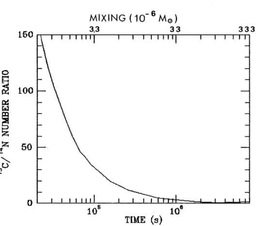
Sy nth esiz ed spectra for H=10-4
CHAPTER 1. INTRODUCTION
1.1) Stellar Neutron Synthesis
Burbidge et al. (1957, hereafter designated B2FH) showed that neutron capture processes have played the primary role in stars of the heavy elements beyond the iron group. Because of repulsive Coulomb forces, charged particle reactions have been rather ineffective at the t empera ures t · (108 to 10 9 oK) at which the main line heavy element synthesis has apparently occurred. It was suggested by Suess and Urey (1956) and Coryell (1956), and shown in detail by B2FH that two quite different and independent neutron capture processes are necessary to synthesize the abundant heavy elements. In one of these processes called the s-process, the neutron captures occur at a slow (s) rate compared to the intervening beta decays. Thus the ~nthesis path lies along the bottom of the valley of mass stability and in general by-passes both the proton rich, lightest isotopes and the neutron rich, heaviest isotopes of the elements involved. On the other hand, in the second neutron process, called the r-process, the neutron capture processes occur at a rapid (r) rate compared to the intervening beta decays. The captures lead rapidly from stable seed nucl ei,
56
occur at quite different rates, then two separate and distinct stages of stellar evolution are required. B2FH assigned the s-process to the red giant stage of stellar evolution and the r-process to events taking place in exploding envelopes or cores of supernovae. The s-process is believed to operate at neutron densities of typically 107 neutrons/cm3 (Blake and Schramm 1975), while the r-process occurs at
neutrons/cm3 (Clayton 1968).
More recent work of neutron ~nthesis in stars has been based upon the identification of a new site for s-process synthesis. This site is the convective helium shells accompanying helium shell flashes in low and intermediate-mass Asymptotic Giant Branch (AGB) stars (Schwarzschild and Harm 1965,1967). Two possible neutron sources first identified by Cameron (1955,1960), the
13C(~,n)160
and the 22Ne (o{,n)25Mg source can be produced in substantial quantities in the convective intershells of such stars. Neutron production via the 13c
source is thought to more 1 ikely oc cur in low-mass (M<
2M ) AGB stars and has been investigated o by Sanders (1967), Cowan and Rose (1977), Despain (1977) and Then and Renzini (1982b). The 22Ne source is believed to be more dominant in the intermediate stars (2M o<
M<
8M ), and the operation of this source in0
such stars has been studied extensively by Iben (1975a, b) and Truran and Iben (1977).
repeating helium shell flashes can lead quite naturally to an exponential distribution of neutron exposures to iron seeds (Ulrich 1973). Seeger, Fowler and Clayton (1965) pointed out that ilie
solar-system heavy element abundances were well modelled by such an exponential exposure. The work of Truran and Iben (1977) indicates that the 22Ne source is the more attractive of the two neutron sources for production of the solar system abundances, mainly due to the filtering action of the progeny of the 22Ne source (see later). Also, the intermediate-mass stars, in which the 22Ne source operates, are thought to contribute substantially to the enrichment of the interstellar medium (Iben and Truran 1978).
the calculations were stopped after 10 6 s. The heavy element enhancements were calculated analytically and as such did not allow the inclusion of the important effect of nuclear branching (see later). It
would be important to extend these calculations to a much wider range of condi tions applicabl e to AGB evol ution. In particular, it would be important to investigate the neutron production resulting from smaller hydrogen mixing events which occur when a full convective link up does not occur. Also, the calculations should investigate the effect of higher base temperatures, and the heavy element network should include nuclear branching if a comparison with observed enhancements is to be of any value.
In order to investigate in detail the parameters which effect neutron production in a low-mass AGB star a light particle network larger than any previously used was constructed. This network was coupled directly to a large heavy element network which included nuclear branching for the element region of interest. The stellar model used was appropriate to a 1.45M AGB star undergoing mass loss via stellar
o
1.2) Discovery of Extremely Hydrogen Deficient Stars
The first extremely hydrogen deficient star was discovered by Popper in 1942 (HD124448). On analysis of this star he found that there were no lines of hydrogen in the visible spectrum and that the lines originally attributed to hydrogen were due to neutral helium. This discovery led to a search by Thackeray and Wesselink (1952) for stars with similar properties. As a consequence of this search, they discovered the hydrogen deficient star HD168476. This was followed by the discovery of hydrogen deficiency in HD160641 by Bidelman (1952). Gould et al. (1957) discovered the first subdwarf (BD+750325) to be deficient in hydrogen,and a year later Greenstein and Wallerstein (1958) found a member of the mul tiple ( j Ori E system was hydrogen deficient
although not to the same extent as the earlier discoveries. This star
is often regarded as the prototype star of the group of stars known as the intermediate helium-rich stars. Another group of stars discovered to be hydrogen deficient are the helium-rich close binaries (Hack 1967) •
B. The helium rich subdwarfs have similar hydrogen abundances to the intermediates and are usually of spectral ~pe
o.
The EHe stars are mostly found at high galactic latitudes, whereas the intermediate helium stars are found in the galactic plane. In general the EHe stars have high galactic latitudes although Hunger (1975) shows that these stars follow the galactic rotation and so the stars may not be necessarily be population II objects as suggested by their high radial velocities. They have present masses in the range 0.6M to 1M with their initial<:> <:>
masses thought to be in the range of 0.9M to 2.1M (Heber 1983). The <:> <:>
difference in these masses being accounted for by stellar wind. The EHe stars and the intermediate stars are not thought to be linked by evolution and it is thought that they form completely independent groups of stars. The hydrogen deficiency of the intermediate helium-rich stars has been suggested by Osmer and Peterson (1974) to be due to diffusion and gravitational settling. The hydrogen deficiency of the helium-rich close binaries is believed to be related to mass transfer mechanisms (Hack 1967). The subdwarfs are not believed to be genetically linked with the EHe stars, however,at the present it is not yet clear whether
the subdwarfs are related to the intermediates.
Warner (1967) included some of the hot EHe stars in his list of cool hydrogen deficient carbon (HdC) stars. These HdC stars can be further divided into variable and non-variable HdC stars. The variable stars are more commonly known as the R Coronae Borealis (RCrB) stars. These stars are believed to be old disc population stars (although the dangers of assigning such a small sample of stars to one particular population should be stressed) with masses similar to those of the EHe stars They are found in the spectral classes F-K and they too are
4
flows onto the RerB star causing the large light variations. But studies of the RerB star RY Sgr (Feast 1978), which also happens to be a pulsating variable with a period of
38.6
days (Alexander et ale 1972), show the infra-red excess of this star also has this period. This would tend to support the idea of a dust cloud intrinsically linked to the star. The known RerB stars are listed in table 1.2.Known EHe stars
star R.A. Dec Mag
BD +31 ltlt2 1 55 36 +38 19.5 10.0
BD +31 1911 9 21 17 +36 55.0 10.1 BD +10 2179 10 36 17.2 +10 19 21 10.0 CPD -58 2121 10 lt5 58.1 -58 53 01 10.3 AE 1 13 20 49.1 -41 28 56 13 - 11 HD 124448 14 11 46.6 -46 03 22 10.0 CoD -48 10153 15 35 24.3 -48 26 14 11.4
HD llt49ltl 16 06 23 -21 08.9 8
BD -9 4395 16 25 51.6 -9 12 54 10.6 V652 Her 16 45 45.9 +13 20 51 10.6 HDE 320156 11 34 31.5 -35 21 21 9.8 V2016 Oph 11 38 55.0 -11 55 00 9.9 LS IV -1 2 11 lt8 51.0 -1 lt2 3lt 11.0 BD -1 3lt38 18 01 20.5 -1 00 33 10.lt
HD 168lt16 18 18 59.8 -56 39 15 9.4 LS IV -14 109 18 56 lt9.1 -14 30 30 11.2 LS II +33 5 19 43 23.1 +33 51 05 10.4 BD +1 lt381 20 lt8 49.5 +2 01 29 9.1
Table 1.2
Known RCrB stars
Star R.A. Dec. Mag
XX Cam It olt 46.1 +53 13 44 8.2- 10.3 W Men 5 21 05 -11 13.6 13.8->18.3 SU Tau 5 46 09 +19 03.1 9.1- 16.0 UW Cen 12 ltO 26 -5lt 15.3 9.6->13 Y Mus 13 02 34 -65 14.1 10.5- 12.1 S Aps 15 Olt 20 -11 52.0 9.6- 15.2 R CrB 15 46 30.1 +28 18 32 5.8- llt. 8
RT Nor 16 20 Olt -59 13.9 11. 3- 16.3 RZ Nor 16 28 39 -53 10 11.1- 12.1 LR Seo 17 2lt 17 -43 48.4 10.9- 12.3 WX CrA 18 05 21 -31 20.1 11.0->16.5 VZ Sgr 18 11 51 -29 lt3.lt 11. 8-> llt • 0 RS Tel 18 15 01 -lt6 3lt. 0 9.3->13.0 GU Sgr 18 21 12 -24 16.8 11.3- 15.0 V348 Sgr 18 31 18.2 -22 51 18 10.6- 11 MV Sgr 18 ltl 32.9 -21 00 21 12.1- 15.6 V CrA 1 8 ltlt 01 -38 12 51 8.3->16.5 SV Sge 19 05 58 +11 32.9 11. 8- 16.2 RY Sgr 19 13 16.8 -33 36 41 6 - 11 U Aqr 22 00 36 -16 52.2 10.5->1lt.lt
.,
a
::>
t z
" 10
..
:t
"'
.. 11 :l
..
:;
2420000 141$000 24]0000
JUliAN DAYS
Figure 1.1 Light curve of HerB (taken from Glasby 1968)
0
~.O~
~~
1
V
/
2
EHe
Red
Giants
0'1
3
8'
-
4
5
H-MS
6
7
White Dwarfs
5'0
4-5
4,0
3-5
log Teff
1.3) Evolution of EHe Stars and HCrB Stars
Schonberner (1975,1977) has suggested the HCrB stars may be the progenitors of the EHe stars. Evidence for this, apart from the obvious similarity with respect to hydrogen deficiency can be found from a study of where these stars are placed on the log g-log Teff diagram. The parameters, gravity and effective temperature are used because they are directly obtained from a fine analysis of the atmosphere without taking recourse to the· mostly ill-defined distances and luminosities of both the HCrB and EHe stars. The g, Teff plane is morphologically a Hertzsprung-Hussell diagram. A line of constant luminosity for a given
2 4 2 4
mass is transformed by Lo(H Teff and go< 1/H to gc( T
eff• From figure 1.2 it can be seen that the HCrB and the EHe stars lie on a line of roughly constant luminosity. This may be an indication of an evolutionary link between the two groups (Schonberner 1977). Also shown in the diagram is the position of the white dwarfs, the hydrogen main sequence and the hypothetical helium main sequence. The EHe star B0+1303224 is not shown here as this star is relatively hydrogen rich compared with other EHe stars and is thought to be in a different evolutionary phase (Jeffery 1984).
not very different to the predicted death rate of EHe stars, so that a large number of all low-mass stars pass through the RCrB-EHe phase. Bues (1970),however,claims that a metal deficiency of 10 to 100 observed in the DB white dwarfs rule out aQY connection with the EHe stars which have a much higher metal abundance. The rapid evolutionary timescales of a few thousand years at the RCrB-EHe phase of evolution would account for the few number of stars observed. Further evidence for a link between the RCrB and the EHe stars is indicated from variability studies of these stars (see section 1.6).
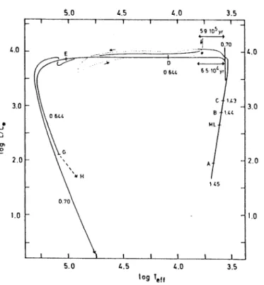
Even if this evolutionary scheme for the RCrB and the EHe stars is correct the problem of explaining the extreme hydrogen deficiency of these objects remains. This has remained the most outstanding problem concerning these stars since Popper's original discovery. It would seem very unlikely for the objects all to have been originally formed from hydrogen free material. The more plausible explanation is that the stars have evolved to their current evolutionary state, either by converting their hydrogen envelopes to helium by complete mixing, or by ejection of the envelope, or by a combination of both. Schonberner (1979) has evolved low-mass AGB models from the early stages of the AGB where helium shell flashes (Schwarzschild and Harm 1965,1967) commence, through to the phase where the models approach the white dwarf regime. A track from these models is shown (full line) in figure 1.3 (the dashed track is due to a possible mixing mechanism discussed in section 1.4). The model commenced with an initial total mass of 1.45M o and an initial helium core mass of M :0.475M. c This represents a post
0
CD -I "--I
en
.Q
4.0
3.0
EHe's
X
loop? / / ./ ./
X
RCrB's
X
/
/
/
2.0
""'''
-_
..
...
","-'1.0
5.0
Figure 1.3
AGB
4.5 4.0
log Teff
1.45M evolutionary track
<:>
the 'hydrogen envelope mass, M (in solar masses), at different phases of e
the stars evolution, having taken account of the stellar wind, is indicated. Also shown is the observed position of the HerB and the EHe stars. It was found that the hydrogen envelope can never be completely removed by this means. This is consistent with a problem first discussed by Packzynski (1971) in attempting to explain the hydrogen deficiency of HerB stars simply by continual mass loss or ejection. The problem being if that such mass loss occurred from the envelope then a compact helium - rich stellar core remai ns. I t is difficu1 t to envisage circumstances which would allow such a remnant core to expand to the high luminosities and large radii found for the HerB stars.
1.4) "Mixing Mechanisms
There is good evidence for some sort of mixing process taking place in red giants in general. This evidence takes the form of the anomalous abundances of carbon and various other chemical elements seen in the atmospheres of these stars. These anomalous abundances suggest that somehow, material which has undergone nuclear burning processes, have been transported to the surface. There have been several models put forward which attempt to explain the mixing processes going on within these stars. Most of these models depend on thermal instabilities in evolved stars. These instabilities are the helium core flash
(discovered by Scbwarzschild and Selberg 1962; Schwarz schild and Harm 1962), and the helium shell flash (discovered by Schwarzschild and Harm 1965,1967). A full review of the abundance anomalies and mixing mechanisms in red giants is given by Scalo (1980).
The helium core flash occurs when helium is ignited in a degenerate core at the tip of the first red giant branch just prior to the horizontal branch phase of evolution. This has been shown to occur in stars with masses less than 2.2M when the core mass reaches 0.45M o
0
After the core flash subsides the star becomes a stable helium core burning object on the horizontal branch. After a period of about 105 years helium is burning in a thin shell surrounding an inert C/O core. Further out in the star hydrogen re-ignites, also in a thin shell, the star is now said to be in a double shell source structure and starts to commence its rise up the AGE. The luminosity of the star arises mainly from the hydrogen shell at this phase of quiescent burning. Depending on the conditions of the helium burning shell (mostly the thickness of the shell) a thermal instability can occur within it. A thermal runaway ensues within the helium shell which causes a rapid rise in the helium shell luminosity (this is termed a "helium shell flash", or a "thermal pulse") • One of main consequences of this luminosity rise is the appearance of an intershell convective zone rising upwards from the helium shell. If this convective zone can reach up to and penetrate the hydrogen shell then the possibility of mixing between the envelope and the interior can occur. The interior structure of the star at this stage for a 1.45M model is shown in figure 3.1
o
detail in chapter 3.
and is discussed in
In intermediate-mass stars the explanation of nuclear synthesized material appearing in the star's atmosphere is more readily explained. Following a thermal pulse (pulse powerdown phase) in such stars, when the hydrogen shell is extinguished, the base of the convective envelope of the star can penetrate down into the carbon-helium rich region left behind by the now extinct convective intershell zone (Iben 1975a,1976,1977). Hydrogen is then mixed into this carbon rich region and freshly synthesized material (i.e. carbon and other nuclei produced in the intershell) can be "dredged up" to the surface. However,in low-mass AGB stars (M
<
2M )0 the convective envelope does not penetrate deep enough for any dredge up to occur. The smallest mass for which the dredge up phenomenon has been found in any calculations is that of Wood's ( 1982) model which had a core mass M =o.67M and a total mass of
c 0
M=2M •
o Further, it is suggested that as the total mass of the star decreases, the minimum core mass for convective dredge up increases (Wood 1981). Yet recent observations of carbon stars in the Magellanic Clouds (eg. Richer 1981) suggests that some form of dredge up occurs in any AGB star irrespective of its mass (Iben 1982). This discrepancy led Iben and Renzini (1982a,1982b) to Show that mixing could arise when the effects of the increased opacity of carbon (generated by the flash) in the cooler regions of the intershell is considered. This increased opacity forms a semi-convective region at the outer edge of the carbon rich region which pushes the carbon rich region further outwards. This new extension of the carbon rich region now enables the base of the convective envelope to make contact with this carbon region, thus enabling a dredge up phenomenon. Iben (1983) further shows that this dredge up in low-mass stars only works for low metallicity and low total
Renzini (1979,1981) has also proposed a mechanism for mixing at a post-AGB phase. This arises from a final helium shell flash which causes total mixing of a small residual hydrogen envelope. The energy generated by the hydrogen burning in the intershell region of the star causes an expansion back to the RerB regime as shown in figure 1.3 (dashed track) • This "loop" mechanism offers an explanation for both the hydrogen deficiency and the large radii (roughly 100R ) observed for e the RerB stars. Such total mixing can occur when the envelope mass Me
<
10- 4M (Fujimoto 1977; Schonberner 1979; Iben et al. 1983) since fore
such a low value of M the entropy barrier discussed by Iben (1976) no e
longer exists. However, such an expansion and subsequent evolution following the loop will be very rapid and this leads to ,difficulties in , accounting for the observed number of RerB stars. So it is clear that the problems surrounding the RerB and the EHe stars are far from being fully resol ved.
enhancements that arise from such mixing can then be compared with observations of these stars.
1.5) Abundance Analyses
Several of the EHe and the RerB stars have had their atmospheres analysed in order to determine their abundances. These abundance analyses used either a coarse analysis or a fine analysis technique. Aller (1954) used the technique of Unsold to do a coarse analysis of HD160641. He found helium, carbon, nitrogen and neon all overabundant with respect to oxygen. Klemola (1961) analysed BD+1002179 and found the carbon and nitrogen abundances normal. HD124448 and HD168476 were analysed in detail by Hill (1965). Hill found both stars overabundant in helium, carbon, nitrogen and possibly neon. Oxygen in HD168476 was verified to be underabundant by Hill (1970). The technique of fine analysis was first applied to BD+1002179 by Hunger and Klinglesmith ( 1969) • Schonberner and Wolf (1974) performed a fine analysis upon HD124448. They also did a differential analysis upon HD168476 relative to HD124448 using Hill's (1964) equivalent widths. Walker and Schonberner ( 1981) re-analysed HD168476 using the fine analysis technique. BD-904395 was also analysed by Kaufmann and Schonberner ( 1977) using the same technique. Recently, BD+10 2179 has been o re-analysed by Heber (1983) using both ultraviolet as well as visible spectra. He also re-analysed HD168476, HD124448 and BD-904395 but this
time including effects of line blanketing as well as using up to date
vary by up to 1.2 dex from star to star. All the stars are carbon overabundant by a factors of roughly 5 to 10 and oxygen underabundant by similar factors (relative to solar values). The elements of the iron group are so far extensively analysed only in the case of HD168476 and BD+1002179 and differ by a substantial amount (Heber 1983): the heavy elements are by more than ten times more abundant in HD168476 than in
With regard to the RCrB stars the first analysis was that of Searle ( 1961) for RCrB itsel f. This was followed by Danziger (1965) for RY Sgr, and Orlov and Rodriguez (1974) for XX Cam. Schonberner (1975) re-analysed all three stars using the previously published data. These abundance analyses were based largely upon relatively strong lines in
.
in fact occurred in at least one of the RCrB stars (see chapter 2).
It is found that the EHe stars are C, Nand 0 poor relative to the RCrB stars. I f the EHe stars are evolved RCrB stars perhaps a better similarity in composition should be observed. However, it is clear that at the present time there is too little abundance data available for any positive conclusions to be made. The possibility exists that the chemical composition of both classes span a broad range and that similarities will emerge only when a larger sample of these objects have been analysed.
1.6) Variability
EHe stars show complicated light and radial velocity variations which make period determinations difficult and which are likely to mask any period changes arising from evolutionary changes in the star. Landolt's (1975) 0.1 day period for BD+13 3224 remains the only EHe star observed o to have a well defined period. Hill et al. (1981) showed that the variations were due to radial pulsations of the star. Kilkenny and Lynas-Gray (1982, 1984) subsequently found the pulsation period to be decreasing at a rate of 4.6xl0-10days/cycle. But as stated earlier this star is thought to be in a different phase of evolution from the other EHe stars (Jeffery 1984). Walker and Kilkenny (1980) suggest that variability will be a common feature amongst EHe stars.
minimum light following one of its rapid declines in brightness. Very high frequency pulsations in HCrB were not detected by Horowitz (1971) in 1969. There are suggestions that the pulsations of HY Sgr may die out from time to time (Mayall 1972) and also those of HCrB (Fernie 1972). It is also suggested that the pulsation amplitude may be largest during the recovery from minimum for UW Cen (Bateson 1972).
It was suspected by Gough (Trimble 1972) that hot helium rich stars would be in an instability strip. The calculations were made mainly for HCrB stars and thus at cooler temperatures than required for the EHe stars. It appeared that there would be an instability strip at around
o
7850 K for Z=0.03. A lower metal abundance would bring the start of this instability region up to higher temperatures. Wood (1976) found an overtone instability region occurring between 5500 oK and 13000 oK (depending on LIM). There was also a tendency for instability to occur around 16000 oK. The importance of investigating the pulsation periods in HCrB and EHe stars is two-fold. Firstly, it is possible to derive a distance-independent mass estimate for stars which pUlsate. Secondly, changes in the pulsation periods of these stars can be compared with the values anticipated from the evolutionary tracks of Schonberner (1977). Kilkenny (1982) and Marraco and Milesi (1982) have indeed demonstrated that the pulsation period in HY Sgr is decreasing at a rate comparable with that expected for Schonberner's (1977) evolving 1M hydrogen
o
1.7) Plan Of Thesis
CHAPTER 2. BASIC NUCLEOSYNTHESIS THEORY
2.1) Nuclear Reactions in Stellar Interiors
a) Generalities
A brief introduction on nuclear processes in stellar interiors is presented here. A more complete description can be found in Fowler et a1. (1967, 1975) and Chiu (196S). The Maxwellian averaged product,<a v>, of the reaction cross section, a , and the relative velocity, v, for two interacting nuclei is
1I2
J
00«(]"v> = (S/i!') a(E) E exp(-E/kT)dE M1/2(kT)3/2
o
(2.1)
where M is the reduced mass, k the Boltzmann constant, T the temperature and E the relative energy of the particles. It is convenient to write the number densities as
( 2.2) 3
where
f
is the mass density (g/cm ), NA is Avogadro's number, Xi is the mass fr'action of nuclei i, and Ai is the atomic mass of i in AMU (Atomic Mass Units). The mean lifetime, t2(1) of nucleus 1 for interaction with nucleus 2 is given by
'Consider the reaction whereby particles 1 and 2 form particles 3
and 4 with an energy release of Q (i.e. an exothermic reaction; for an
endothermic reaction Q will be negative), viz. 1+2
->
3+4+Q. Since itmay be easier to measure a required cross section in the reverse
direction, use is frequently made of the reciprocity theorem, which
follows from the assumption of time-reversal invariance for the nuclear
and electromagnetic interactions (e.g. Blatt and Weisskopf 1952, Fowler
et al. 1967)
~(34) _ (1 + ~34) g1 g 2A1A2E12 ~(12) (1 + 612) g3g 4A3 A4E34
where
l
is the Kronecker delta, g.=(2J.+1) is the statistical weight of~ ~
nucleus i with spin J
i , A1 is the reduced mass of particle in AMU
(similarly ~, A3 and A4), and E12 and E34 are the kinetic energies in
the centre of mass system on the two sides of the nuclear equation. The
introduction of the (1+
b)
term reflects the fact that cross sectionsbetween identical particles are twice those between different particles,
other factors being equal. Since Q=E
34-E12 it is easily found from
equation 2.1 that
<34>
-<12>where
This equation applies to nuclei which are in their ground states only.
In nuclear processes at high temperatures, such as those found in
important part in the reaction. In most cases of interest the excited states of the nuclei will be in equilibrium with the ground state. A
*
test can be made by comparing the lifetime t(i->i ) for photoexcitation from the ground to the excited state, with the time
astrophysical circumstance under consideration.
I
*
scale, t , of
a the
Equilibrium will be obtained for t(i->i ) < t . The lifetime t(i->i ) can be computed from
a
*
the spontaneous decay lifetime of the excited state t sp (i ->i) which can be calculated (Fowler et al. 1967) by using
I
t (i->i )
*
t (1->1)sp
= gi [exp(Ei*/kT) - 1] gil
(2.4)
where Eil is the excitation energy of the excited state and T is the
*
ambient temperature. The effects of induced emission on i ->i were incorporated by the incl usion of the -1 in equation 2.4. For the case of reactions involving all the exci ted states of the nucl ei in equilibrium with the ground states, equation 2.3 is modified by replacing the gi by the nuclear parti tion functions
=
t
g,*exp(-Ej*/ kT)j*
*
where the sum over i includes the ground state and runs through all
*
excited states for t(i->i )<t
a• The rare situation where a long lived excited state is not in thermal equilibrium is important. The importance of these isomeric nuclei is discussed later. A frequent use of the reciprocity theorem is in the measurement of photodisintegration of nuclei at temperatures T6>500 (in this notation T6 signifies units of However, since the reactions to be considered in this thesis will b~ at temperatures T6<300 the photodisintegration of nuclei will
The effect of electron screening was first discussed by Salpeter (1954). This screening is due to the electrons in the ionised gas of a stellar interior, reducing the effective electrostatic repulsion of two nuclei. An ion in a plasma is surrounded by a charge cloud of radius which is of the order of the Debye length, L
d, where
r.
2.11/2Ld =~T/(41Yne
)J
and where n is the electron density. The electrostatic potential between two nucl ei is
VCr) (2.5)
where r is the distance between the nuclei, u(r) is the screening correction to the coulomb potential Z1Z2e /r and u(r) varies with the 2 characteristic length r
char• The classical turning radius r c for two bodies interacting through the coulomb interaction is
2
rc = Z1 Z2e
E
where E is the relative particle energy. For the conditions of low dens; ty r ... , c
<...
• char· Therefore s; nce u(r) only changes significantly ... over r char' then u(r ) = u(O) = constant = U • c 0 Using equation 2.5 as the new potential i t is found that the reaction rate is given byThe effect of electron screening is therefore the same as introducing a correction factor exp(-U /kT).
The best method for evaluating the integral in equation 2.1 depends on the type of energy dependence exhibited by a-(E). Several commonly occurring cases will now be considered.
b) Non-Resonant Reactions
In the first approximation the effect of electron screening is ignored. Consider two particles with charges Z1 and Z2' and separated by a distance r (the situation of reactions involving neutrons is discussed later). The electrostatic potential energy is given by
2
V(r)
=
Z1 Z2 e rThe probability of a nuclear reaction can be written as the product of the probability P
L (Coulomb penetration factor) that the two particles approach one another at a distance r=R (where L is the relative angular momentum of the nuclei and R is the minimum radius of interaction;
1/3
R=1.4A fm), and the probability P nuc that the particles in contact react in a nuclear fashion. The first stage is illustrated in figure 2.1. I t is clear that for the nuclear reaction to proceed the particles must penetrate the coulomb barrier, the height of which is given by
2
Ec = Z1 Z2e R
quantum mechanical effect of tunnelling gives the probability that the particles with relative energy E approach, by a tunnel effect, the interaction radius R. The Coulomb barrier penetration factors were first discussed by Gamow (1928), and Gurney and Condon (1928,1929). The penetration factor P
L is given by P
L =
[F~(R)
+G~(R)]-1
(2.6)where FL(R) and GL(R) are the regular and irregular solutions of the Schrodinger wave equation for a charged particle in a Coulomb field evaluated at the interaction radius R. The Coulomb wave functions FL(R) and GL(R) are discussed and tabulated by Froberg (1955) and Hull and Breit (1959). Approximate values of the penetration factors are derived using the WKB (Wentzel 1926; Kramers 1926; Bri1lioun 1926) solution to the Schrodinger equation (cf. Bethe 1937, Van Horn and Salpeter 1967). The WKB solution for P
L is
(2.7)
where each symbol is as before and ~ is the rationalised Planck constant. For low energy reactions (E«E )
c L=O and it can be seen that
1-211Z1Z2e~
E-1/2t
1i
vj
If the factor P nuc is more or less independent of the energy of the . incident particle then
<T (E) = PLP v-1 = S(E) E-t . exp [-(E IE) 1/2]
nuc G (2.8)
where EG is the Gamow energy and is given by
The factor SeE) (in units of MeV-barns) is termed the 'astrophysical factor' • It measures the probability of the purely nuclear reaction, and is usually measured experimentally by means of the inverse formula
1/2
SeE)
=
~ (E) E exp [(Ea/E) ]Far from a nuclear resonance SeE) is a slowly varying function and it may be conveniently expressed in terms of the power series expansion
SeE)
=
5(0)
[I
+
(2.9)where a prime denotes differentiation with respect to the kinetic energy E in the centre of mass system.
The reaction rate r12 for a non-resonant charged particle reaction between nuclei 1 and 2 will be
r 12 = N1N2 <O"v>12
(1 +612)
where N1 and N2 are the number densities given by equation 2.2. It follows from equations 2.8 and 2.1 that
y
S [
~E
)Vl.
E
J
N,Nl.
(~)2.
_,
3SeE) exp -
~
- -
clE
1+ dl1..
ffM
(kT)
V'l.E
k1
(2.10)
Using equation 2.9 Bachall (1966) and Fowler et al. (1975) evaluated the' integral to show
(2.11)
In this equation, E is
energy, corresponding to the peak in the integrand of equation 2.10, 6E o is the full width of this effective energy peak at 1/e maximum value, Seff is the effective value of the cross section factor S(E), and T co is the cut-off temperature which occurs when the nuclear cross section no longer varies according to the Coulomb penetration factor (this condition may occur when the effective energy Eo is larger than EG 01" when the continuum 01" a resonance has set in - see later). Eo is given by (Fowler and Hoyle 1964)
Eo = ['1(0<. Z1 Z2kT (Mc 2/2) 1/2]2/3
and 6E is given by o
t:. E = 4 (E kT 13) 1 12
o 0
(2.12)
(2.13)
The effective value Seff of the cross section factorS(E) is given by
(2.14)
Equation 2.14 will give Seff in units of MeV-barn. Equations 2.2, 2.12, 2.13 and 2.14 can be combined to give the useful result
-C T-1/3 _
2 9 (T I T )
2
] {1 + C T 1 1 3 + C 4
~91
3
9 co 3 9
where
+ C T5/3 }
7 9
C
1
=
7.8324x10⁹(Z~Z;A)1/6S(O)/A1/2,
C2
=
4.2475(Z~Z~A)1/3,
C3
=
9.810X10⁻²(Z~Z~A)-1/3,C
4
= O.1220{S'(O)/S(O)} (Z~Z~A)1/3,-2 C
5
=
8.377x10 S'(O)/S(O), C6
=
7.442x10⁻³ {S"(0)/S(0)} (Z2 Z2 A) 2/3 1 2 ' C7
=
1.229x10⁻²{S"(0)/S(0)} (Z2 Z2A) 1/3 1 2 't
Energy
/
Nucleus
Figure 2.1
t
CT (E)
TunneL
f
E
!
R r
-Tunnelling effect of particle with E
<
E cMuLt Iresonant
-enveLope
Figure 2.2
. /
///t
Non-resonant
envelope
Energy _
c) Resonant Reactions
For a single resonance of energy E
R, the cross section cr(E) of the nuclear reaction 1+2
->
3+4+Q is given by (Breit and Wigner 1936)0-
(E)
==
(2.15)where E is the is the centre of momentum energy of 1 and 2 and
i\
=1'1/ (Mv) (where M is the reduced mass)is the reduced de Broglie wavelength. The statistical factor w is given bywhere J is the angular momentum of the resonant state and where J
1 and
J
2 are respectively the angular momentum of particl es and 2. The total width
r
of the resonant state is given byr
=fl/t , where t ise e
the effective lifetime of the state. The partial width
r
12 is the width for re-emission of 1 and 2,and
t;4
is the width for emission of 3 and 4. The partial widths can be evaluated using the expression(2.16) where R is the interaction radius P
L is the Coulomb penetration factor given by equation 2.6 and e~ is the reduced width for particles with angular momentum L. It follows from equations 2.15, 2.10 and 2.1 that for a resonant reaction in a non-relativistic, non-degenerate gas the reaction rate 1"12 is given by
When the effective energy E given by equation 2.12 is much smaller than o
the resonant energy E
R, then the Breit Wigner resonant cross section may
be evaluated in its wings to give the cross section factor
S( E) = 0.657 w
G
2 ( E)1;
4 expA (E- ER ) 2 + (
r
2 Ill)(2.18)
S( E) is in MeV barns and E in MeV. Equation 2.18 may be evaluated using measurements of a resonance at high energies, and then used with the
no~resonant formalism of equations 2.11 and 2.111 to obtain reaction rates at low energies. When the range of effective stellar energies
includes the resonance energy then equation 2.17 must be used. This is
provided that the width of the resonance,
r,
is much less than theeffective spread in energy of the interacting particles (i.e. less than
6E). Equation 2.17 can be integrated to give o
3 -1 -1
cm sec (mole)
where (2.19)
11 -3/2
r.
C8 = 1.53986x10 A w 12 ~lI/r ,and
C
9=11.605 ER•
The effect of a single resonance is included in the tabulations of
N A
<
(J' v> referenced for the no~resonant reaction rates. When severalsuperposition
' \ -3/2
NA<O"v> = ~C8nT9 exp (-C9
i
T9) (2.20)where C
8n and C9n are the appropriate constants given by equation 2.19
for the nth resonance. When the density of resonances lying within 6E o
becomes sufficiently large the summation of equation 2.20 can be
replaced by the integration dE/D, where D is the average level distance
within the Gamow peak. This occurs mainly in elements heavier than
about Neon In this situation where the resonances are so closely
spaced such as to form a continuum of resonances, the reaction rate
takes the same form as the non-resonant case. This is to be expected
since at that time the average behaviour of the nucleus is relatively
independent of the energy. The' average properties of the nuclei
required for this statistical analysis of the reaction rates are usually
calculated by using a Wood-Saxon optical potential (Michaud et al.
1970) for the nuclei. Such an analysis was carried out by Holmes et
al. (1976) and Woosley et al. (1978) for a large number of heavy
nUclei. The O"(E) behaviour for the different cases discussed here is
illustrated in figure 2.2.
d) Neutrons
The reaction rates for neutron absorption reactions follow the same
analysis as given in the previous sections only this time there is no
need for the Coulomb penetration factor since the neutron carries zero
electric charge. For non-resonant reactions the energy dependence of
( 1964) • At low energies the s wave (L=O) interactions dominate and the cross section is proportional to the square of the de-Broglie wavelength
?\
and the partial width for neutron emissionr.
n Since
X
isproportional to v-1 while
~
is proportional to v, v being the relative veloci ty of the neutron and interacting nucl eus, i t follows that for norr-resonant neutron reactions (J' 0<. V -1 or (J'v=constant. The Maxwellianaveraged cross section is defined as
where is the most
<0') = <(J'v)/v
T
probable velocity of the Maxwell-Boltzmann distribution and is given by
v
T = (2kT/M) 1 12
Measurement of neutron cross sections are usually taken at the most probable
section Values
energy (=kT), then
<
(J' )=O"T taken at vT• Values of the cross 8 (J'T are measured at 30keV or T
8=3.48, that is vT=2.4x10 cm/s. at other temperatures are then extrapolated using the relationship v-1 T 0<.. T -1/2 • In some cases the thermal neutron cross section O"Th is given. These cross sections are measured at T=293 oK , that is at kT=O.025 eV. For resonant and continuum neutron reaction rates the analysis follows that given for the charge particle reactions but wi th the
replaced by kT.
e) Beta Decay
Individual stellar transition rates for electron emission, positron emission, continuum electron capture and K electron capture may be calculated from an expression of the form
A
=I
n 2 f( Z ,w )
- - 0
<ft)
where f(Z,W ) is the Fermi function characterising the transition, Z is o
the charge of the parent nucleus and VI 0 is the maximum energy release of
the beta decay. <ft>=f(Z,Vl
o)t1/2 (where t1/2 is the beta decay half life) is a factor which is found to be roughly constant for any given degree of forbiddenness of the beta transition. For the different beta processes a different expression is used in order to calculate the Fermi function. In the case of the electron or positron
Wo
j
PE(E-Wo)2F (± Z,E)dE f
=
1m5c9 meL.
emission this is
where p is the electron (positron) momentum, m is the electron rest mass, c is the velocity of light and where the + and - signs correspond to the cases of electron and positron emission respectively. The function F(!
z,
E') corrects for Coulomb effects on the electron(positron) wavefunction and is given by (e.g. Blatt and Weisskopf 1952) • The integrated Fermi function for K-capture can be found from the relativistic formula (Blatt and Vleisskopf 1952)
fk = 21r (2p )2S-2 ~(12S+1(Wo+s)2
where
y
= Rmcib,
'(f
=
0<. z,2 1/2 s = (1- { ( z-1) o(} )
r::
is the Gamma functionand where d... is the fine structure constant and R is the nuclear radius. Newman (1973) has shown how to correct the experimental terrestrial rates for K-capture for the effects of ionisation of K electrons. For continuum electron capture the appropriate function f was approximated
ec by Bachall (1962) and is given there.
The above expressions can be used to calculate the individual transition rates of stellar beta decays. Laboratory <ft> are usually used when possible, otherwise 'average' <ft> values appropriate to a given degree of forbiddenness are adopted. Data required for the excited states of the parent nucleus can be found from Nuclear Data Sheets (Volume 26). The total decay rates are determined by summing over all individual excited state contributions weighted by the appropriate statistical factor, i.e.
where
A
total =L.
Pi'LAi, ji
J
Pi
=
20i + 1) exp(-Ei/kT) , Uenergy E.) of the parent nucleus, and U is the partition function. ~
Tables of stellar beta decays for a large number of nuclei which were calculated using the methods outlined here are given in the tables of Newman (1973) and Cosner (1982).
2.2) Heavy Element Synthesis by the S-Process
Merrill's (1952) discovery of Technetium in the atmospheres of red-giant stars is generally accepted as evidence that neutron capture processes are significant with regard to heavy element ~nthesis in the interiors of stars. This is because the longest lived isotope of Technetium (99Tc ) has a terrestrial half life of 2x10⁵years. Since this is short compared to the stellar lifetime it follows that Tc must be produced in the star. Also since the energies of the nuclei in a stellar interior are too low for charge particles to have any effect on Tc production (due to the Coulomb barrier) it follows that neutron absorption reactions must be at work.
The slow neutron capture process, 01'" s-process, for the production
2
the time between successive neutron captures on a given nucleus is of
the order of hundreds to thousands of years, and that the s-process is
characterised by a low neutron density (roughly 107 neutrons/cm3, Blake and Schramm 1975). I f it is assumed the beta decays of unstable nuclei occur much more rapidly than the neutron captures then the
nuclear network can be represented by a linear chain in which there is
only one nucleus for each value of atomic number A. The number
abundance of any nuclide, Nit (the notation Nit is used here so as to
avoid confusion with Avogadro's number), is then determined by the set
of equations
(2.21 )
A = 57,58, ••••••••
where N is the neutron number abundance and assuming the lightest n
nucleus in the capture chain is 56 Fe • The reaction rate <(J'v> can be
factorised into < (J' > and v 1/2
T=( 2kT/M) • By defining a neutron exposure, ~ , by
t
r
=
i
NnvTdt ,o
the equations 2.21 may be written in the form given by CFHZ
d~,
0-; ~
d
<;1"
cr",d.1"
where
YI
(2.22)
- 4\,+
tf/<-I ,k = 2,3 , ••••••••and
trK
=-
Zo->A
NA
N;6
and
N~6
is the initial 56 Fe abundance. An exact solution to the~stem
of equations 2.22 was known from the work of Bateman (1910). This gives the abundance of any nuclide Nl as a function of the neutron exposure '/, in the form( 2.23) where
C
A .,L.
0-.;-, (J":r+ . • . • . . . ' . (JA
However, there are two severe difficulties with this exact solution. The functional form is incorrect for aQY two cross sections which are equal, and secondly, even for cross sections which have similar values (which is frequently the case) then the CA,i's are difficult and time consuming to evaluate numerically. These difficul ties led CFHZ to approximate equations 2.23 for <J"ANA by,
rr1 -/
N;6 AA
(AAI)
Ae.~
p
c-
A/l1'-)
r;,
(mil)
where
fy
is the gamma function and11 A 1..
All
-
-
L6Ycr~
n1A
--(r
Y
at )
L~n11
I
Ycr..'L
( L
Y"iJ
• C. I--;c,6
distribution of neutron exposures found to observed solar system abundances was found weighting function of the form
R('! ) = G exp (-7'/'1
0)
where R(i'"") is the fraction of the material exposure
'I,
and G and1"
o are constants.give a best fit to the to be an exponential
having received a neutron
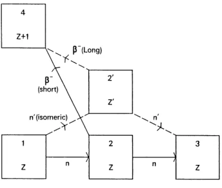
Although satisfactory for qualitative descriptions, this formulism is not satisfactory for detailed quantitative calculations of individual nuclei, especially for high neutron densities. The problem is that the phenomenon of rruclear branching cannot be included in any lineal" network. Nuclear branching is illustrated in the full lines of figure 2.3 (the dashed lines and primed nuclei are related to isomerism, see later) • Nucleus 1 absorbs a neutron and form nucleus 2. Now nucleus 2 is unstable and can beta decay forming nucleus 4 in a short time. If however nucleus 2 absorbs a further neutron in a time scale similar to its beta decay, then some fraction of nucleus 2 will form nucleus
3.
There is then a branch in the flow chart. The amount of flow passing through nucl ei 3 and 4 will then depend on the neutron densi ty, and the neutron absorption cross section and the beta decay rate of nucleus 2. Further neutron absorption on nucleus 4 will then mean that two different nuclei in the network now possess the same atomic mass A.