Using volunteered geographic information (VGI) in design based statistical inference for area estimation and accuracy assessment of land cover

Using Volunteered Geographic Information (VGI) in Design-Based Statistical Inference 1

for Area Estimation and Accuracy Assessment of Land Cover 2

3

Stephen V. Stehmana_{, Cidália C. Fonte}b_{, Giles M. Foody}c_{, Linda See}d 4

5 6

a_{Department of Forest and Natural Resources Management, SUNY College of Environmental Science} 7

and Forestry, Syracuse, NY 13210, United States (svstehma@syr.edu) 8

9

b_{Departmento de Matemática, Faculdade de Ciências e Tecnologia, Universidade de Coimbra, Apartado} 10

3008, EC Santa Cruz, 3001 – 501 Coimbra, Portugal (cfonte@mat.uc.pt) 11

12

c_{School of Geography, University of Nottingham, Sir Clive Granger Building, University Park,} 13

Nottingham, NG7 2RD, United Kingdom (giles.foody@nottingham.ac.uk) 14

d_{International Institute for Applied Systems Analysis (IIASA), Schlossplatz 1, A-2361 Laxenburg, Austria} 15

(see@iiasa.ac.at) 16

17

Corresponding Author:Stephen V. Stehman (svstehma@syr.edu) 18

19

Abstract 20

Volunteered Geographic Information (VGI) offers a potentially inexpensive source of reference data for 21

estimating area and assessing map accuracy in the context of remote-sensing based land-cover 22

monitoring. The quality of observations from VGI and the typical lack of an underlying probability 23

sampling design raise concerns regarding use of VGI in widely-applied design-based statistical inference. 24

This article focuses on the fundamental issue of sampling design used to acquire VGI. Design-based 25

inference requires the sample data to be obtained via a probability sampling design. Options for 26

incorporating VGI within design-based inference include: 1) directing volunteers to obtain data for 27

locations selected by a probability sampling design; 2) treating VGI data as a “certainty stratum” and 28

augmenting the VGI with data obtained from a probability sample; and 3) using VGI to create an 29

data that were obtained from a non-probability sampling design, but require additional sample data to 32

be acquired via a probability sampling design. If the only data available are VGI obtained from a non-33

probability sample, properties of design-based inference that are ensured by probability sampling must 34

be replaced by assumptions that may be difficult to verify. For example, pseudo-estimation weights can 35

be constructed that mimic weights used in stratified sampling estimators. However, accuracy and area 36

estimates produced using these pseudo-weights still require the VGI data to be representative of the full 37

population, a property known as “external validity”. Because design-based inference requires a 38

probability sampling design, directing volunteers to locations specified by a probability sampling design 39

is the most straightforward option for use of VGI in design-based inference. Combining VGI from a non-40

probability sample with data from a probability sample using the certainty stratum approach or the 41

model-assisted approach are viable alternatives that meet the conditions required for design-based 42

inference and use the VGI data to advantage to reduce standard errors. 43

44

Key Words: probability sampling; external validity; pseudo-weights; data quality; model-based 45

inference; Volunteered Geographic Information (VGI); crowdsourcing 46

47

1. Introduction 48

Volunteered Geographic Information (VGI) is defined as “tools to create, assemble, and 49

disseminate geographic data provided voluntarily by individuals” (Goodchild 2007). For land-cover 50

studies, VGI may provide the reference condition or the information used to determine the reference 51

condition of a spatial unit. The reference condition, defined as the best available assessment of the 52

ground condition, plays a critical role in accuracy assessment and area estimation (Olofsson et al. 2014). 53

When used in map production, VGI could form all or part of the data used to train the land-cover 54

accuracy assessment and area estimation. Accuracy assessment is an essential component of a rigorous 56

mapping-based analysis of remotely sensed data as without it the obtained products are little more than 57

pretty pictures and simply untested hypotheses (McRoberts 2011; Strahler et al. 2006). In addition an 58

accuracy assessment adds value to a study, especially when estimates of class area (e.g. deforestation) 59

are to be obtained (Olofsson et al. 2014). Fonte et al. (2015) examined the use of VGI for land cover 60

validation, including the types of VGI that have been used, the main issues surrounding VGI quality 61

assessment, and examples of VGI projects that have collected data for validation purposes. We build 62

upon this past work to focus on the issue of statistical inference when incorporating VGI in applications 63

of accuracy and area estimation, but our work is also relevant to application of citizen science data in 64

general (Bird et al. 2014). 65

Map accuracy assessment is a spatially explicit comparison of the map class label to the 66

reference condition on a per spatial unit basis (e.g., pixel, block, or segment). Accuracy assessment 67

typically focuses on producing an error matrix and associated summary measures including overall, 68

user’s, and producer’s accuracies (see Section 2 for details). Estimates of area of each land-cover class 69

or type of land-cover change based on the reference condition are often produced in conjunction with 70

the accuracy estimates (Olofsson et al. 2013, 2014). Sampling, defined as selecting a subset of the 71

population, is almost always necessary because it is too costly to obtain a census of the reference 72

condition. VGI represents a subset of the population and as such may be viewed as a sample. Whether 73

the VGI data were collected via a probability sampling design is a key consideration when evaluating the 74

utility of VGI for design-based inference. Design-based inference is a standard, widely used approach 75

adopted in environmental science for furthering knowledge and understanding on the basis of a sample 76

of cases rather than a study of the entire population. 77

We describe options for incorporating VGI into map accuracy assessment and area estimation 78

VGI can be transformed into more precise estimators (i.e., smaller standard errors, a desirable outcome 80

of an effective sampling strategy) within the scientifically defensible framework provided by design-81

based inference. If the VGI data are obtained via a probability sampling design, application of design-82

based inference is straightforward and can be informed by good practice guidelines (Olofsson et al. 83

2014). Alternatively, if the VGI data are not obtained via a probability sampling protocol, the VGI data 84

can be combined with additional data from a probability sample to produce estimates that satisfy the 85

conditions underlying design-based inference. In such cases the VGI data from a non-probability sample 86

serve as a means to reduce standard errors of estimates rather than as the sole data from which the 87

area and accuracy estimates are produced. 88

89

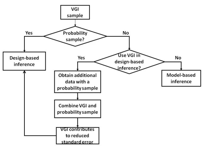
Figure 1. Schema for methodologies using VGI in accuracy assessment and area estimation. 90

91

This article has two major objectives. First, it illustrates how statistically rigorous and credible 92

inference may be drawn from studies that use VGI and thereby helps ensure that the vast potential of 93

potential as a source of land cover information which is often constrained by lack of ground reference 95

data. Second, the article provides methodological rigor and good practice advice for the use of data 96

acquired via popular sample designs, ranging from judgmental to probability sampling. As such this 97

article articulates methodology for producing credible inference from data sets that often do not 98

conform to the requirements of widely used statistical inferential methods for two common and 99

important application areas of remote sensing, accuracy assessment and area estimation. To do this, 100

we, for the first time, synthesize methods developed in the general sampling literature into a 101

comprehensive treatment of the theory and methods for using VGI in design-based inference. This 102

includes translating methods developed for the use of non-probability samples for accuracy assessment 103

and area estimation applications. As such we will show how VGI may be constructively used to decrease 104

costs and reduce uncertainty (e.g., yield smaller standard errors and hence narrower confidence 105

intervals) while following a methodology that allows for rigorous design-based inference. Throughout 106

this article, guidance for using VGI in design-based inference is framed by examining the direct 107

connection of the inference process to the three component protocols of accuracy assessment, the 108

response design, sampling design, and analysis (Stehman and Czaplewski 1998). 109

The article is organized as follows. In Section 2, we define inference and describe the conditions 110

needed to satisfy design-based inference. Considerations regarding the use of VGI in design-based 111

inference are then explained in Section 3 in regard to the response design, sampling design and analysis 112

protocols. Section 4 provides the details of two methods for incorporating VGI in estimation of accuracy 113

and area that satisfy conditions of design-based inference, with both methods requiring that an 114

additional probability sample exists or could be acquired if the VGI did not originate from a probability 115

sampling design. Options for analysis when the only data available are VGI from a non-probability 116

sample are discussed in Section 5. Sections 6 and 7 provide discussion and a summary of the article. 117

119

2. Inference 120

Following Baker et al. (2013, p.91), we define statistical inference as “… a set of procedures that 121

produces estimates about the characteristics of a target population and provides some measure of the 122

reliability of those estimates.” Statistical inference focuses on the use of sample data to estimate 123

parameters of a target population, where a parameter is defined as a number describing the population 124

(e.g., the population mean and population proportion are two common parameters). Determining the 125

numerical value of a parameter would require a census of the study region, but in practice parameters 126

are estimated from a sample. Statistical inference also includes how bias and variance of these sample-127

based estimators are defined. Baker et al. (2013, p.91) further specify that “A key feature of statistical 128

inference is that it requires some theoretical basis and explicit set of assumptions for making the 129

estimates and for judging the accuracy of those estimates.” Consequently, sampling design and analysis 130

protocols must adhere to certain rules of implementation to ensure that the underlying mathematical 131

basis of the inference framework is satisfied. Failure to adhere to these rules may lead to substantial 132

bias in the estimators of parameters of interest or even nullify the ability to implement design-based 133

inference entirely (see Section 3.3). 134

Two general types of inference are design-based inference and model-based inference (De 135

Gruijter and Ter Braak 1990; Särndal et al. 1992; Gregoire 1998; Stehman 2000; McRoberts 2010, 2011). 136

In design-based inference, bias and variance of an estimator are determined by the randomization 137

distribution of the estimator which is represented by the set of all possible samples that could be 138

selected from the population using the chosen sampling design. This randomization distribution is 139

completely dependent on the sampling design hence the origin of the name “design-based” inference. 140

that underlies design-based inference (Särndal et al. 1992, section 2.4). The practical considerations for 142

using VGI in design-based inference are explained in detail in Section 4. 143

A probability sampling design must satisfy two criteria related to the inclusion probabilities 144

determined by the sample selection protocol. The inclusion probability of a particular element of the 145

population (e.g., a pixel) is defined as the probability of that element being included in the sample. An 146

inclusion probability is defined in the context of all possible samples that could be selected for a given 147

sampling design. For example, if the design is simple random sampling ofnelements selected from the 148

Nelements of the population, the inclusion probability of each elementu of the population is πu=n/N. 149

That is, in the context of all possible simple random samples of sizenfrom this population, elementu 150

has the probability ofn/Nof being included in the sample selected. The two requirements of a 151

probability sampling design are that πu must be known for each element of the sample and πu>0 for 152

each element of the population (Särndal et al. 1992; Stehman 2000). Probability sampling requires a 153

randomization mechanism to be present in the selection protocol. Convenience, judgment, haphazard, 154

and purposive selection of sample elements are examples of protocols that do not satisfy the criteria 155

defining a probability sampling design (Cochran 1977, Sec. 1.6). Use of such samples for inference 156

carries considerable risk due to lack of representation of the population. 157

An alternative to design-based inference is model-based inference (Valliant et al. 2000). As the 158

name implies, model-based inference requires specification of a statistical model and inference is 159

dependent on the validity of the model. Consequently, verifying model assumptions is a critical and 160

often challenging feature of model-based inference. Model-based inference does not require a 161

probability sampling design, although implementation of a probability sampling design is often 162

recommended to ensure objectivity in sample selection because of the randomization (Valliant et al. 163

2000, p.20). Applications of model-based inference are briefly discussed in Section 5.3. 164

166

3. Component Protocols of Accuracy Assessment and Area Estimation 167

We describe the role of each of the three components of the methodology (response design, 168

sampling design, and analysis) in determining how VGI can be incorporated in rigorous design-based 169

inference. The response design is the protocol for determining the reference condition (i.e., the best 170

available assessment of the ground condition). The response design includes all steps leading to 171

assignment of the reference condition label of a point or spatial unit (e.g., a land-cover class or change 172

versus no change label). The sampling design is the protocol for selecting the sample units at which the 173

response design will be applied. Lastly, the analysis consists of defining parameters to describe 174

properties of the population (e.g., overall accuracy, proportion of area of each class) and the formulas 175

required to estimate these population parameters from the sample data. To justify the requirements of 176

each step to achieve the final accuracy or area estimates, our description starts with the analysis 177

(Section 3.1) focusing on how the VGI data would be used, followed by the steps of the response design 178

(Section 3.2) and the sampling design (Section 3.3). 179

180

3.1 Analysis: Accuracy and Area Estimation Based on Totals 181

The details of the analysis protocol that specify how the estimates of accuracy and area are 182

produced yield insights into how VGI should be evaluated for use in design-based inference. The 183

analysis focuses on summarizing information contained in an error matrix. We define the population to 184

be a collection ofNequal-area units partitioning the region of interest. The population error matrix 185

resulting from a census can be constructed in terms of area as illustrated by the numerical example in 186

Table 1 for a simple two-class legend, “crop” and “not crop” for a population (target region) of 1000 187

km2_{. The error matrix expressed in terms of area (Table 1) could easily be converted to proportion of} 188

matrix expressed in terms of area because we can formulate the population parameters of interest for 190

accuracy and area as totals or ratios of totals of areas. For example, overall accuracy is the total area of 191

agreement obtained from the sum of the area of the diagonal cells (930 km2_{) divided by the total area of} 192

the target region (1000 km2_{) to yield overall accuracy of 0.93 or 93%. User’s accuracy for the crop class} 193

is the total area where both the map and reference condition are crop (840 km2_{) divided by the total} 194

area mapped as crop (890 km2_{) to yield the parameter 0.94 or 94%. Producer’s accuracy for the crop} 195

class is the total area where both the map and reference condition are crop (840 km2_{) divided by the} 196

total area of reference condition of crop (860 km2_{) to yield the parameter 0.98 or 98%. Lastly, the area} 197

of reference condition of the crop class is also simply a total, in this case the sum of the two cells in the 198

“crop” column of reference condition (840+20 = 860 km2_). 199

200

Table 1. Population error matrix expressed in terms of area (km2_{) for a hypothetical target region of} 201

1000 km2_{. Overall accuracy is 93% (930/1000).} 202

Reference Condition 203

Map Crop Not Crop Total User’s

204

Crop 840 50 890 0.94

205

Not Crop 20 90 110 0.82

206

Total 860 140 1000

207

Producer’s 0.98 0.64

208 209

Given that the parameters of interest for accuracy and area can be expressed in terms of totals, 210

the analysis focuses on estimating these totals. Basic sampling theory provides an unbiased estimator of 211

a population total in the form of the Horvitz-Thompson estimator (Horvitz and Thompson 1952). The 212

ܻ=∑௉ݕ௨ [1]

214

where the summation is over allNelements of the population,P. For example, ifyuis the area of crop 215

(as determined from the reference condition) for elementu, thenY is the total area of crop. The 216

population totalYcan be estimated from a sample using the Horvitz-Thompson estimator 217

ܻ෠=∑ ௬ೠ గೠ

௦ [2]

218

where the summation is over all elements of the samples. 219

The Horvitz-Thompson estimator is an unbiased estimator of a population total for any sampling 220

design as long as the inclusion probabilities of the sample elements are known for that design. A useful 221

re-expression of the Horvitz-Thompson estimator highlighting the sample estimation weights is 222

ܻ෠=∑௦ݓ௨ݕ௨ [3]

223

wherewu = 1/πuis the estimation weight for elementuof the sample. Becausewu≥1, theyuvalue for 224

each sampled element is multiplied by an “expansion factor”wuto estimate a total. In effect each 225

sample element must account for itself along with some additional elements of the population that 226

were not selected into the sample. For example, for simple random samplingwu=N/nsoyufor each 227

sampled element is “expanded” by the multiplierwuto account forN/nelements of the population. The 228

critical importance of known inclusion probabilities for rigorous design-based inference is evident via 229

the role of the weightswu = 1/πuin the estimatorܻ෠(equations 2 and 3). 230

Parameters such as user’s accuracy and producer’s accuracy are ratios of totals and 231

consequently can be estimated by the corresponding ratio of estimated totals (Särndal et al. 1992, 232

section 5.3). For example, if we defineYas the total area of the population for which both the map and 233

reference condition are crop andXas the total area mapped as crop, the ratio of population totalsY/X 234

would be the population parameter for user’s accuracy of crop. User’s accuracy could then be estimated 235

from the sample data using a ratio of Horvitz-Thompson estimators,ܻ෠/ܺ෠, where bothܻ෠and ܺ෠are 236

reference condition of crop andxu=area of pixelumapped as crop. In the case of a pixel-based 238

assessment and assuming all pixels are equal area, user’s accuracy of crop estimated using a ratio of 239

Horvitz-Thompson estimators would simply require definingyu=1 if pixeluhas both map and reference 240

labels of crop (yu=0 otherwise) and definingxu=1 if pixeluhas map label of crop (xu=0 otherwise). In this 241

formulation of user’s accuracy, the ratioY/Xis the proportion of pixels mapped as the target class that 242

have the reference label of that class. 243

Formulas for the variance and estimated variance of the Horvitz-Thompson estimator are 244

provided by Särndal et al. (1992, section 2.8). The square root of the estimated variance (standard 245

error) would be used to construct a confidence interval for the parameter of interest so issues of 246

inference obviously extend to variance and confidence interval estimation. Although we do not delve 247

into the details of the formulas for variance estimators, we emphasize that known inclusion probabilities 248

are an essential feature of variance estimation. Consequently, the requirement of implementing 249

probability sampling to ensure known inclusion probabilities for estimating a total applies as well to 250

estimating the variance of an accuracy or area estimator. 251

The conditions required for VGI to be used in design-based inference are apparent from the 252

analysis protocol. The accuracy and area parameters of interest can be expressed as population totals 253

or ratios of population totals and these totals can be estimated using the Horvitz-Thompson estimator. 254

From the Horvitz-Thompson estimator formula (equations 2 and 3) we observe that the key features of 255

VGI relevant to estimating a total are quality of the observationyuand knowledge of the inclusion 256

probability πu. In other words, the questions pertinent to evaluating the utility of VGI for design-based 257

inference are: 1) What is the quality ofyu (an issue to address in the response design) and 2) Is πuknown 258

(an issue to address in the sampling design)? The following two subsections address issues of VGI 259

related to the response and sampling designs. 260

3.2 Response Design 262

The response design is the protocol for determining the reference condition of an element of 263

the population. In the case of a land-cover legend based on a conventional hard classification, the 264

response design results in a reference land-cover label assigned to each pixel (i.e., if the legend consists 265

ofCclasses, one and only one of these class labels is assigned to the pixel). The reference class labels 266

can be translated to a quantity by the simple process of definingyu= 1 if pixeluhas reference classcand 267

yu= 0 otherwise. Thus for example if classcis forest, all pixels with reference class forest would be 268

assignedyu= 1 and all non-forest pixels would haveyu= 0. Evaluating and assuring the quality of VGI is 269

critical because high quality reference data are absolutely essential to accuracy and area estimation. If 270

the reference labels are not accurate, these errors can have a substantial impact on accuracy and area 271

estimates (Foody 2009, 2010). Very accurate reference data obtained within a timeframe corresponding 272

to the date of remote sensing image acquisition are a necessity for every application of accuracy 273

assessment and area estimation from remote sensing. VGI has considerable potential as a source of 274

reference data, notably in facilitating the collection of a large set of observations over broad 275

geographical regions. However, the use of volunteers rather than experts in assigning the reference 276

class labels may exacerbate concerns regarding label accuracy, although amateurs can sometimes be as 277

accurate as experts in labeling (See et al. 2013). Further, VGI tends to be collected continuously rather 278

than within a narrow time frame which can limit its value, especially for studies of land-cover change. 279

Applications in which VGI has been collected for land cover and land use studies are becoming 280

increasingly common. Fonte et al. (2015) reviewed several applications including: 281

1) Geo-Wiki project, which uses the crowd for interpretation of very high resolution satellite 282

imagery (Fritz et al. 2012); 283

3) geo-tagged photographs for land cover validation from different applications such as the 285

Degree Confluence Project, Geograph, Panoramio and Flickr (Antoniou et al. 2016; Fonte et al. 286

2015; Iwao et al. 2006). 287

Another source of VGI for land-cover studies is the LACO-Wiki system, an online land cover validation 288

tool intended as a repository of openly available validation data crowdsourced from different users (See 289

et al. 2017). More recently, land cover and land use have been crowdsourced in the field through the 290

FotoQuest Austria app, which sends users to specific locations and loosely follows the LUCAS protocol 291

for data collection (Laso Bayas et al. 2017). Hou et al. (2015) describe geo-tagged web texts as an 292

alternative to photographs as yet another source of VGI useful for land-cover studies. 293

The quality of the VGI data collected for land cover and land use studies has received recent 294

attention. A substantial body of literature focuses on the positional quality and completeness of 295

OpenStreetMap (OSM), the most commonly cited VGI project (e.g., Ciepłuch et al. 2010; Girres and 296

Touya 2010; Haklay 2010). Other elements of quality include thematic accuracy (which is relevant to 297

land cover and land use), temporal quality, logical consistency, and usability, all of which are set out in 298

ISO 19157 (Fonte et al. 2017a). In addition, Antoniou and Skopeliti (2015) outline quality indicators that 299

are tailored to VGI such as data indicators, demographic and other socio-economic indicators, and 300

indicators about the volunteers. Due to the specificities of VGI when compared to traditional 301

geographic information and the diversity of uses of these data, additional methodologies are starting to 302

be developed that aim to integrate several quality measures and indicators into quality assessment 303

workflows, enabling quality data to be combined to produce more reliable quality information (e.g., 304

Bishr and Mantelas 2008; Jokar Arsanjani and Bakillah 2015; Meek et al. 2016). 305

Although concern with reference data error may be heightened when VGI is used, there are 306

methods such as latent class analysis, which can be used to characterize volunteers in terms of their 307

subsequently in applications (Foody et al. 2013, 2015). These issues of data quality associated with the 309

response design are critical to the overall process of accuracy and area estimation. In reality, reference 310

data quality issues are equally impactful whether the source of the reference classification is VGI or 311

expert interpretation (See et al. 2013). 312

313

3.3 Sampling Design 314

The sampling design is the protocol used to select the subset of locations (e.g., pixels) at which 315

the reference condition is determined. As noted earlier, the inclusion probability of pixeluis denoted as 316

πu, and the two criteria defining a probability sampling design are: 1) πuis known for all pixels in the 317

sample and 2) πu> 0 for all pixels in the population. Because probability sampling is a requirement of 318

rigorous design-based inference, the sample selection protocol must ensure that these two conditions 319

of πuare satisfied. Moreover, randomization of the sample selection is required of all probability 320

sampling designs as it is this randomization that creates the probabilistic foundation for design-based 321

inference. The sampling design is linked to the analysis via the inclusion probabilities that are 322

incorporated in the Horvitz-Thompson estimator (equations 2 and 3). 323

Because design-based inference requires known inclusion probabilities, it is critical to establish 324

whether a probability sampling design was the basis for collecting VGI data. The distinction between 325

active and passive VGI is relevant in this regard. Active VGI refers to directing volunteers to specific 326

sample locations (e.g., See et al. 2016) and therefore allows for implementing a probability sampling 327

design for collecting VGI. Conversely, passive VGI refers to allowing volunteers to choose where they 328

will collect data and typically leads to purposive or convenience sampling with attendant concern 329

regarding lack of representation of the full population. The protocols that determine where VGI data 330

are collected span a continuum ranging from rigorous probability sampling to selection by judgment or 331

The Degree Confluence Project (Iwao et al. 2006) is an example in which VGI data are collected 333

via a probability sampling protocol. These data are obtained at locations defined by the intersection of 334

lines of latitude and longitude and therefore originate from a design akin to systematic sampling (due to 335

the Earth’s shape the distances between sample points vary with latitude so the inclusion probabilities 336

would not all be equal but would still be known). A second example of VGI based on a probability 337

sampling design is the FotoQuest Austria app which uses the Land Use/Cover Area frame Survey (LUCAS) 338

sample (which is based on a systematic sample of points spaced 2 km apart in the four cardinal 339

directions across the European Union) followed by a stratified sample (Martino et al. 2009). That is, land 340

cover and land use were crowdsourced via the FotoQuest Go mobile app in which volunteers were sent 341

to specific locations that formed part of the LUCAS systematic sample for Austria, and the LUCAS sample 342

was then augmented with additional sample units (Laso Bayas et al. 2016). 343

Several VGI applications include sample data originating from both probability sampling designs 344

and volunteer chosen locations. The Geo-Wiki project is used to collect land cover and land use data via 345

different campaigns (See et al. 2015). These campaigns have all had different purposes and hence were 346

driven by different sampling designs. For example, the first campaign to validate a map of land 347

availability for biofuels was driven by a stratified random sample with equal sample size in both the land 348

available stratum and the land unavailable stratum. To this an additional sample from cropland areas 349

was added although the data were not used to undertake an accuracy assessment as such but to modify 350

the statistics on how much land is available (Fritz et al. 2013). Other studies have made use of Geo-Wiki 351

data from previous campaigns for validation that were not obtained using a probability sampling 352

approach for the specific product to be validated (see, for example, Schepaschenko et al. (2015) and 353

Tsendbazar et al. (2015) for review of reference datasets including those from Geo-Wiki). The VIEW-IT 354

application (Clarke and Aide 2011) either directs users to specific locations selected based on a 355

means these latter sample locations would not be part of a probability sampling design. The LACO-Wiki 357

system (See et al. 2017) has built-in probability sampling schemes although users can upload their own 358

sample locations that do not necessarily conform to a probability sampling design. 359

Photograph repositories such as Panoramio, Flickr, and Instagram are examples of passive VGI 360

and therefore do not conform to any probability sampling design. For example, photographs made 361

available by citizens may be positioned at any location chosen by the volunteer (such as the 362

photographs available in Flickr or Instagram), or collected at predefined locations. Similarly, the data 363

available in collaborative projects such as OSM are created at locations of interest to the citizen 364

volunteers, and consequently these data have no underlying probability sampling design. The amount 365

and quality of the OSM data are known to be correlated with demographic or socio-economic factors 366

(e.g., Mullen et al. 2014; Elwood et al. 2013) and this offers some possibility for adjusting estimates to 367

account for misrepresentation of the population (see Section 5.1). 368

The Geograph project asks users to take photographs in every square kilometer of the United 369

Kingdom and classify them (now also extended to other locations in the world). Since 2005, 83.4% of 370

the 1 km2_{squares in Great Britain and Ireland have photographs (http://www.geograph.org.uk/,} 371

accessed 29 October 2017) and nearly 5.5 million images are available within this time period. 372

Volunteers may choose locations within each square kilometer at which photographs are taken. 373

Therefore, if each photograph is viewed as representing a point location or, for example, the 30 m x 30 374

m pixel surrounding the photograph’s location, the data would not meet the criteria defining a 375

probability sampling design due to the lack of randomization in the selection protocol. Directing the 376

volunteers to cover the 1 km2_{squares provides a better degree of spatial representation of the VGI than} 377

might otherwise occur if volunteers are allowed to choose locations completely on their own. 378

Specifically, the 1 km2_{squares effectively serve as spatial (geographic) strata, and with over 83% of} 379

well distributed (Stehman 1999, Figure 3). The Geograph project data collection protocol illustrates the 381

fact that within the class of non-probability sample designs, features can be built into the protocol to 382

enhance representation of the VGI data. 383

384

4. Methods to Use VGI in Design-based Inference 385

In this section, we address how to incorporate VGI into design-based inference focusing on 386

sampling design and estimation considerations (Figure 2). The label quality issues of VGI remain a 387

concern but are not addressed in this section. The most straightforward approach to ensure the utility 388

of VGI for design-based inference is to direct volunteers to collect data at locations specified by a 389

probability sampling design (which is possible with “active VGI”). Several examples of VGI collections 390

based on a probability sampling design were documented in Section 3.3. Specifying sample locations 391

selected via probability sampling has the potential drawback that volunteer participation may be 392

reduced if volunteers are unable to choose locations of personal interest. Consequently, additional 393

effort may be necessary to obtainyuat those locations neglected by volunteers. 394

396

Figure 2. Schema for using VGI in design-based inference. 397

If a large quantity of VGI obtained from a non-probability sampling design exists, the VGI data 398

may be augmented with data from a probability sampling design (Figure 2). Two options are described 399

in the following subsections. In the first option, the VGI data are treated as a “certainty stratum” and 400

combined with data from a probability sample selected from the locations not already included in the 401

VGI data. In the second option, the probability sample is selected from the full population and the VGI 402

data are used to construct an auxiliary variable that is then incorporated in a model-assisted estimator 403

to reduce the standard errors of the estimates based on the data from the probability sample. 404

405

4.1 VGI Incorporated as a Certainty Stratum 406

VGI data can be combined with data obtained from a probability sample by treating each VGI 407

sample unit (e.g., a pixel) as belonging to a “certainty stratum” in which the inclusion probability is πu=1 408

(Overton et al. 1993). By assigning πu=1 to each VGI sample unit, we acknowledge that these sample 409

been purposely selected to be included with certainty in the sample. From the remaining units of the 411

population not included in the VGI certainty stratum, a probability sampling design is implemented and 412

these newly selected sample units are combined with the VGI data to produce the accuracy and area 413

estimates. In this approach the VGI data are used directly in the estimation of accuracy and area, so the 414

quality of the VGI data is a critical concern. 415

All sample units selected via the probability sampling design will have a known inclusion 416

probability and the data from these sample units can be combined with the VGI data using the Horvitz-417

Thompson estimator. Specifically, suppose there areN1elements for which we have no VGI andN2 418

elements for which VGI providesyu(N=N1+N2). Further, letGdenote the subset for which VGI is 419

available (the “G” is from the middle letter of VGI) andܩ෨denote the subset of the population for which 420

VGI is not available. The population totalYcan then be partitioned into summations over the two 421

subpopulationsܩ෨andG, 422

ܻ=∑ீ෨ݕ௨+∑ீݕ௨=ܻீ෨+ܻீ [4]

423

BecauseYG(total ofyufor the VGI data) is known, it is only necessary to estimateܻீ෨from the sample.

424

Therefore, an estimator ofYcan be expressed as 425

ܻ෠=∑௦ݕ௨/ߨ௨+∑ீݕ௨=ܻ෠ீ෨+ܻீ [5]

426

where the first summation is over the elements selected in the sample from theN1elements of the 427

populationܩ෨for which VGI is not available. The variance ofܻ෠isܸ൫ܻ෠൯=ܸ(ܻ෠ீ෨)because the total of the

428

VGI data is a known quantity with no uncertainty attributable to sampling. That is, the only uncertainty 429

attributable to sampling arises from estimating the totalܻீ෨for the non-VGI portion of the population,

430 ܩ෨. 431

The benefit of the VGI data when incorporated as a certainty stratum is to reduce the standard 432

errors of the accuracy and area estimators and accordingly to decrease the width of confidence intervals 433

objective of estimating area based on the reference condition obtained for each sample unit. The 435

benefit of the VGI data can then be quantified by comparing the variance of the estimator of total area 436

without using VGI data to the variance of the estimator using the certainty stratum approach (equation 437

5). Several conditions are imposed to simplify the variance comparison: 1) the sample of non-VGI units 438

is selected by simple random sampling; 2) the VGI data have the same variability as the non-VGI data 439

(i.e., the variance ofyufor the VGI subpopulationGis the same as the variance ofyufor the non-VGI 440

subpopulationܩ෨); and 3) the sample sizenis the same regardless of whether VGI is present (i.e., the VGI 441

data are viewed as obtained at no cost sonis the same with or without VGI). If no VGI data are 442

available and a simple random sample is selected from the full population ofNelements (i.e.,N2=0 443

because no VGI data exist), the variance of the estimated total is 444

ܸ൫ܻ෠൯=ܰଶ_{ቀ1 −}௡

ேቁܸ௬/݊ [6]

445

The variance ofܻ෠when VGI is available forN2elements of the subpopulationGis derived as follows. A 446

simple random sample ofnelements is selected from theN1non-VGI units. The variance of the 447

estimated total combining the VGI data with the non-VGI sample (equation 5) depends only on the 448

variance of the total estimated from the non-VGI sample units, 449

ܸ൫ܻ෠ீ෨൯=ܰଵଶቀ1 −_ேభ௡ቁܸ௬/݊ [7]

450

To quantify the reduction in variance achieved by the VGI data, we examine the ratio of the two 451

variances, 452

ܴ=௏൫௒෠ಸ෩൯ ௏(௒෠) =

ேభమቀଵି_{ಿ భ}೙ቁ ேమ_ቀଵି೙

ಿቁ

[8] 453

TheVy/nterm common to both equations (6) and (7) cancels in the ratioRby virtue of the assumption 454

that the variability ofyuis the same in the VGI and non-VGI subpopulations (ifVyis different in the two 455

Under the assumption of equal variance for the two subpopulations, the benefit of VGI to 457

reduce variance depends on the proportion of the population that is covered by the VGI data, which is 458

defined ask=N2/N. If we definef=n/Nto be the proportion of the total population selected for the 459

probability sample, thenRcan be re-written as 460

ܴ= (1 −݇)(1 −݂−݇)/(1 −݂). [9]

461

If no VGI data exist, thenk=0 andR=1 as expected because there would be no reduction in variance 462

from VGI. Conversely, ifk=1, thenR=0 as expected because the VGI would constitute a census and the 463

population totalYwould be known yielding a variance of 0. As the quantity of VGI gets larger (i.e., 464

k=N2/Nincreases),Rdecreases indicating a greater benefit accruing to the availability of the VGI data. 465

Numerical values of√ܴ(ratio of standard errors) for several combinations ofkandfare presented in 466

Table 2. For a fixed value off=n/N,_√ܴdecreases approximately linearly with increasingk. For a fixed 467

value ofk, the decrease in_√ܴis much less prominent asfincreases except for the case withf=0.25 and 468

k=0.75 which represents a census soܸ൫ܻ෠ீ෨൯= 0. To simplify the problem still further, assume that the

469

spatial unit of the assessment is a pixel and thatNis so large thatf=n/N =0. Then settingf= 0 in 470

equation (9), we obtainR= (1 -k)2_{which leads directly to} 471

√ܴ= 1 −݇ [10]

472

Thus for very large populations the reduction in standard error achieved by VGI will be directly related 473

tok, the proportion of the population for which VGI is available – the greater the quantity of VGI 474

available (i.e., largerk) the greater the reduction in standard error. 475

Table 2. Reduction in standard error achieved by using VGI in the certainty stratum approach. Values 480

shown in the table are_√ܴwhere R is the ratio of the variance of the estimated total with VGI data 481

incorporated in a certainty stratum divided by the variance of the estimated total in the absence of VGI 482

(see equations 8 and 9). Ratios are provided for different combinations ofk=N2/N(the proportion of the 483

region of interest covered by VGI) andf=n/N(proportion of the study region covered by the simple 484

random sample). 485

f=n/N 486

k 0.00 0.01 0.05 0.10 0.25 487

0.01 0.99 0.99 0.99 0.99 0.99

488

0.05 0.95 0.95 0.95 0.95 0.94

489

0.10 0.90 0.90 0.90 0.89 0.88

490

0.25 0.75 0.75 0.74 0.74 0.71

491

0.50 0.50 0.50 0.49 0.47 0.41

492

0.75 0.25 0.25 0.23 0.20 0.00

493

0.90 0.10 0.10 0.07 0.00 0.00

494 495

Equation (9) and the results of Table 2 can be used to examine the benefit of VGI arising from 496

photographs contributed by volunteers (Antoniou et al. 2016), a common source of VGI for land-cover 497

studies. Suppose we assume a photograph to be representative of a 30 m x 30 m pixel and consider a 498

region of interest that covers 8 million km2_{(roughly the size of the conterminous United States,} 499

excluding Alaska and Hawaii). This region would have approximatelyN= 9 billion pixels. To achieve a 500

5% reduction in the standard error of the estimated area of a targeted class (i.e.,_√ܴchanges from 1 to 501

0.95) the certainty stratum approach would requirek=N2/N=0.05 which translates to needingN2= 450 502

for VGI data to contribute a 5% reduction in standard error we would needN2= 5 million photographs. 505

Typically the VGI photographs will have to be processed to obtain the land-cover information of interest 506

(e.g., a land-cover class). Consequently, the large number of photographs needed in these examples to 507

achieve only a 5% reduction in standard error would require substantial computer processing capability 508

and possibly automated methods to identify the land-cover class from the photographs. Accordingly, 509

the response design effort to process such large numbers of photographs may make this use of VGI cost 510

prohibitive in some applications. 511

The certainty stratum approach may have greater utility when the VGI data are in the form of 512

fully mapped areas classified to a land-cover or change type (i.e., in contrast to individual, unlabeled 513

photographs as in the previous paragraph). For example, Fonte et al. (2017b) described an application 514

in which OSM provided land-cover information for two study areas of 100 km2_{in London and Paris.} 515

OSM coverage was 88% for the London region and 97% for the Paris region. Because of the substantial 516

portion of area covered by OSM (k=0.88 for London and k=0.97 for Paris) a large reduction in standard 517

error of accuracy and area estimates would be expected by using these OSM data in the certainty 518

stratum approach. For example, ifk=0.88 and f=0.1 (the London example), we obtainR=0.00266 519

(_√R=0.05) indicating that the standard error of the certainty stratum estimator would be 5% of the 520

standard error of the estimated area when not using the VGI from OSM. Obviously the areas of the 521

regions of interest for the OSM examples in this paragraph are much smaller than for the examples in 522

the previous paragraph andkwould surely be smaller if OSM were to be used for national estimates. 523

524

4.2 Use of VGI in a Model-Assisted Estimator 525

Brus and de Gruijter (2003) developed an approach to use data from a non-probability sampling 526

design to produce estimates within the design-based inference framework. In this approach, a spatial 527

variable for allNelements of the population. The auxiliary variable is then used in a model-assisted 529

estimator to achieve a reduction in standard error. Model-assisted estimators represent a broad class of 530

estimators in which one or more auxiliary variables are incorporated in the estimator. Common 531

examples of model-assisted estimators include difference, ratio, and regression estimators as well as 532

post-stratified estimators (Särndal et al. 1992; Gallego 2004; Stehman 2009; McRoberts 2011; Sannier et 533

al. 2014). The auxiliary variables are expected to covary with the target variable of interest and the 534

information in the auxiliary variables, when incorporated in the model-assisted estimator, thus serves to 535

reduce standard errors (Särndal et al. 1992, Chapter 6). 536

The Brus and de Gruijter (2003) approach could be applied to VGI as follows. Consider the 537

objective of estimating the proportion of area of a class (e.g., area of forest) based on the reference 538

condition. Suppose the spatial unit of the analysis is a pixel and the VGI data consist ofN2pixels labeled 539

as forest or non-forest. The Brus and de Gruijter (2003) approach uses these VGI data to construct an 540

auxiliary variablexufor allNpixels in the population. For example, for a binary classification of forest / 541

non-forest, the auxiliary variable would be defined asxu=1 if the class is forest andxu=0 if the class is 542

non-forest. The auxiliary variablexuis known for theN2pixels comprising the VGI, and the Brus and de 543

Gruijter (2003) approach would then implement a spatial interpolation method such as indicator kriging 544

(e.g., Isaaks and Srivastava 1989) to predict values ofxufor theN-N2pixels not included in the VGI subset 545

of the population. The binary forest / non-forest classification of the region predicted from the VGI data 546

could be used in the same manner as auxiliary data from any forest / non-forest map. For example, to 547

estimate the proportion of area of forest based on the reference condition (yu), a probability sample 548

from allNpixels would be selected for which the reference class of each sampled pixel would be 549

obtained. If the reference observation is also a binary forest / non-forest classification (i.e.,yu=1 if the 550

reference condition is forest,yu=0 otherwise), an error matrix could be estimated from the sample 551

data. The error matrix information could then be combined with the VGI generated forest / non-forest 553

map information to produce a post-stratified estimator of the proportion of area (Card 1982; Stehman 554

2013). The expectation is that the auxiliary variable created from the VGI would yield a reduction in 555

standard error of the post-stratified estimator relative to an estimator that did not incorporate the VGI. 556

That is, the map generated via spatial interpolation of the VGI data would be used in the same way that 557

a forest / non-forest map derived from remotely sensed data would be used in a post-stratified 558

estimator. 559

The Brus and de Gruijter (2003) method requires a probability sample to provide the reference 560

data (yu) for the accuracy and area estimates. This probability sample must be selected from the full 561

population ofNunits, including those units for which VGI is available. In contrast, the certainty stratum 562

use of VGI (section 4.1) does not require a sample from the subpopulationGthat has VGI. The Brus and 563

de Gruijter (2003) approach does not use the VGI data as the observed response (i.e., the reference data 564

value,yu) so the quality of the class labels associated with the VGI data will not impact the estimates in 565

terms of potential bias attributable to labeling error of the VGI. However, better quality (i.e., more 566

accurate) VGI data would likely yield a greater reduction in standard error in the same manner that a 567

more accurate map yields a greater reduction in standard error when the map data are used in a post-568

stratified estimator (Stehman 2013). In the context of land-cover accuracy and area estimation 569

applications, remote sensing information is almost always available to produce a map that would 570

provide auxiliary information that could be used in a model-assisted estimator. Spatial interpolation of 571

VGI using the methods described by Brus and de Gruijter (2003) provides another option for producing a 572

map of auxiliary information,and incorporating remote sensing imagery in linear spatial models (Diggle 573

et al. 1998) might further enhance the precision benefit of the Brus and de Gruijter (2003) approach. 574

To summarize, the model-assisted estimator based on spatially interpolated data does not rely 575

the concern with bias attributable to inaccurately labeled VGI data. Instead, the approach employs the 577

VGI to create an auxiliary variablexuthat is then used in a model-assisted estimator to reduce the 578

standard errors of the accuracy and area estimates. The magnitude of the reduction in standard error 579

would depend on the quality of the VGI. While this approach would have great utility if no other 580

auxiliary information were available, we typically have access to remotely sensed data that could be 581

used to produce a classification that would serve the same purpose as a map derived from spatially 582

interpolating VGI data. Consequently, for land-cover studies the primary benefit obtained by spatial 583

interpolation of VGI may occur in circumstances where a map produced from remotely sensed data is 584

not available. 585

586

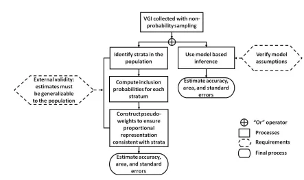
5. Use of VGI from Non-Probability Samples 587

If the VGI data are the only source of reference data (i.e., there is no probability sample and 588

unable to acquire one), it will be challenging to use these VGI data in the manner of design-based 589

inference (Figure 3). One option for using VGI in this context is to replace the estimation weights 590

wu=1/πu(equation 3) by pseudo weights that depend on assuming the sample can be treated as though 591

it had been obtained via a probability sampling design. For example, suppose the reference data for 592

accuracy assessment and area estimation are land-cover interpretations extracted from a non-593

probability sample of photographs. If the inclusion probabilities (πu) of the spatial units represented by 594

these photographs are unknown, one approach to estimate totals is to assume that the VGI locations 595

represent a stratified random sample (see Section 5.1 for details). Using this approach it is possible to 596

construct pseudo-weights such that estimated totals will match known parameters of the population. 597

Although this weighted estimation approach can adjust a VGI sample to achieve estimates that 598

correspond to the correct proportional representation of the population, the question of “external 599

Model-based inference is a second option for using VGI data that were not obtained from a probability 601

sampling design. The application of model-based inference to accuracy and area estimation is discussed 602

in Section 5.3. 603

604

605

Figure 3. Schema for using VGI collected via a non-probability sampling design. 606

5.1 Estimation Based on Pseudo-Weights 607

If the only reference data available for accuracy and area estimation are VGI that did not originate 608

from a probability sampling design, an obvious initial step in the analysis is to examine the proportional 609

distribution of the VGI sample relative to known characteristics of the population. For example, using a 610

land-cover map of the study region, we could compare the proportion of the VGI data found within each 611

land-cover class to the proportion of each class in the entire population. For the hypothetical numerical 612

example of Table 3, the VGI sample shows preferential selection from the developed and crop classes at 613

the expense of representation of the “other” and natural vegetation classes reflecting the relative ease 614

could also be assessed by examining the distribution of distances to the nearest road or distances to the 616

nearest population center. For example, we could compare the mean distance to the nearest road for 617

the VGI locations to the mean distance for allNpixels in the population. If the mean for the VGI 618

locations was less than the mean for the population, this discrepancy would indicate preferential 619

selection of VGI closer to a road. A relevant question is then whether this preferential selection could 620

introduce bias because map accuracy may differ depending on proximity to a road. 621

622

Table 3. Hypothetical data illustrating evaluation of the proportional representation of VGI. The 623

distribution of the percent area of the map classes is compared between the VGI sample (n=100) and 624

the population (i.e., entire region) known from a land-cover map of the study region. 625

626

Area (%) 627

Map Class VGI Population

628

Developed 25 10

629

Crop 35 20

630

Natural vegetation 30 50

631

Other 10 20

632 633

In general, we could attempt to adjust estimates to account for recognized non-proportionality of 634

the VGI data relative to known population characteristics (Dever et al. 2008). For the example data of 635

Table 3, the difference between the distribution of the VGI and population data suggests that weighting 636

the data to adjust for this discrepancy would be a good idea when producing estimates. One approach 637

would be to construct weights such that the estimates based on the weighted analysis of the VGI data 638

sample as having arisen from a stratified design (e.g., Loosveldt and Sonck 2008). Inclusion probabilities 640

for each stratum are then defined asߨ௨=݊௛/ܰ௛wherenhis the observed sample size (from the VGI

641

sample) in stratumhandNhis the population size in stratumh. The estimation weight for pixeluis then 642

ݓ௨= 1/ߨ௨, and these weights could be used in the Horvitz-Thompson estimator. These stratified

643

estimation pseudo-weights for the hypothetical data of Table 3 are presented in Table 4. Referring to 644

weights constructed in this manner as “pseudo-weights” highlights the fact that they are not derived 645

from inclusion probabilities generated by a probability sampling protocol. 646

647

Table 4. Pseudo-weights for VGI sample units based on distributions by class shown in Table 3 (nhand 648

Nhrepresent the number of pixels for each class in the VGI sample and in the population). 649

650

nh Nh

651

Class VGI Map wu=Nh/nh

652

Developed 25 1000 40

653

Cultivated 35 2000 57

654

Natural veg 30 5000 167

655

Other 10 2000 200

656

Total 100 10000

657 658

To illustrate how the stratified estimation approach using pseudo-weights is implemented, consider 659

estimating the proportion of area mapped as the developed class. From Table 3, we know this 660

proportion is 0.10 because we have the map for the entire population. How well does the VGI sample 661

estimate this parameter? We observe that 25 out of 100 VGI pixels are mapped as developed so the 662

parameter of 0.10 for the population. To produce the estimator using the stratified pseudo-weights of 664

Table 4 we defineyu=1 if the sample pixel has the map label of developed andyu=0 otherwise. Then for 665

the developed class stratum,yu=1 for all 25 sample pixels and each of these pixels has a weight of 666

wu=40, so the estimated total contributed from this stratum is 40 x 25 = 1,000 pixels (using equation 3). 667

For the other three strata,yu=0 for all sample pixels so these strata contribute no additional pixels to the 668

estimated number of mapped developed pixels. Dividing the estimated total number of map pixels 669

labeled as developed (1,000) by the number of pixels in the population (N=10,000) yields an estimated 670

proportion of 0.10 which matches the population proportion of mapped developed area from Table 3. 671

Thus the sample estimate using the pseudo-weights matches this known population proportion. 672

In general, the pseudo-weights can be constructed so that the sample estimates will equal known 673

population values. In the example of Table 4, the pseudo-weights reproduce the known values 674

Nh=population size of each stratum, a property known as “proportional representation.” These same 675

estimation pseudo-weights are then applied to estimate the target population parameters and the 676

assumption is that estimation weights that effectively adjust the VGI sample data to match known 677

population parameters will also work well when estimating the target parameters for which we do not 678

have full population information. Other more complex methods for creating estimation weights include 679

raking, general calibration estimators (Deville and Särndal 1992), and propensity scores (Valliant and 680

Dever 2011). Models can be used to produce the pseudo-weights used in lieu of weights that are the 681

inverse of the inclusion probabilities of a probability sampling design, but Valliant (2013, p.108) points 682

out that this approach has not yielded promising results because the models are weak and the 683

requirements excessive for covariates to be used in the models. 684

685

Pseudo-estimation weights can be used to produce estimates that capture the proportional 687

distribution of known population characteristics (i.e., covariates). However, another important aspect of 688

representativeness of non-probability sample data is external validity, defined as the parameter estimates 689

being “generalizable outside the sample, say to the population of interest” (Dever and Valliant 2014). For 690

the pseudo-weight estimation approach described in the previous section, establishing external validity 691

would require that accuracy for the subset of the population represented by the VGI locations be 692

equivalent to accuracy of the full region. Proportional representation of the estimates (Table 4) produced 693

from non-probability sample data is one aspect of external validity, but proportional representation is not 694

sufficient to establish external validity (Dever and Valliant 2014). 695

External validity may also require establishing that the population represented by the VGI is the 696

same as the population of the full study region. Two examples are provided to illustrate this practical 697

issue. In both examples, the objective is to estimate the accuracy of a map. For the first example, suppose 698

that volunteers avoid locations of complex land cover and provide reference data exclusively for locations 699

that are surrounded by homogeneous land cover. Antoniou et al. (2016) suggest such a strategy may be 700

beneficial when using photographs to avoid difficulties of determining the ground condition. Because 701

homogeneous regions are typically more likely to be classified correctly, the accuracy estimates produced 702

from such data would be expected to have higher accuracy than is true of the study region as a whole. 703

Consequently external validity of these data would be suspect because the estimates based on the non-704

probability sample would not be generalizable to the target population. As a second example, suppose 705

because of convenient access the VGI data have been collected primarily at locations near roads. 706

Evaluating external validity would then require determining whether accuracy near roads was equivalent 707

to accuracy distant from roads. 708

Verifying external validity of VGI may be extremely challenging and in some cases impossible 709

characteristics of the full study region. Consider the example of VGI data concentrated along roads. To 711

establish that accuracy does not vary with distance from a road, we could collect additional reference 712

data distant from roads based on a probability sampling design, and compare the accuracy estimates 713

from this sample to accuracy estimates for sample data constrained to locations near roads. But the 714

additional effort to obtain the sample data distant from roads would negate much of the value of VGI 715

for reducing the cost of accuracy assessment. That is, to definitively establish the equivalence of 716

accuracy near roads to accuracy distant from roads, we may need a large probability sample, and the 717

primary value of VGI is to reduce the cost and effort of collecting sample data. 718

Alternatively, it may be possible to cite previous studies to establish external validity. For example, 719

if previous research has demonstrated that distance from a road is not strongly related to accuracy, we 720

would have some assurance of external validity to support use of VGI data collected preferentially near 721

roads. In general, to more fully exploit the potential benefit of VGI, it may be necessary to document 722

typical features of VGI that would commonly need to be addressed to establish external validity and 723

then conduct the necessary studies to inform the decision of whether external validity is tenable. 724

Distance from road, characteristics of volunteers, and complexity of landscape are just a few examples 725

of features that might be explored to determine whether characteristics of populations (e.g., accuracy) 726

differ by these features. If in general there are no such differences, external validity of non-probability 727

sample data is supported to some degree. Developing a cohesive strategy to design and conduct such 728

studies for a broadly applicable assessment of external validity of VGI would likely require a major 729

research initiative. 730

731

5.3 VGI and Model-Based Inference 732

Model-based inference is not predicated on probability sampling so it is a potentially attractive 733

inference requires specification of a model that relatesyuto a set of covariates (predictors) available for 735

the full population (Valliant et al. 2000). Developing appropriate models and evaluating the underlying 736

assumptions may be difficult and time-consuming (Baker et al. 2013) with the difficulties exacerbated by 737

the fact that in most surveys, numerous estimates are produced from a single sample. In the case of 738

VGI, estimates of accuracy and area for several land-cover or land-cover change types will typically be of 739

interest, and each of these estimates may be desired for several subregions within the target region of 740

interest. A model will need to be developed and assumptions evaluated for all estimates as a model 741

that works well for some estimates may not work well for others. An additional challenge to the model-742

based approach is that non-probability samples may have an inherent selection bias, so a substantial risk 743

exists that the distribution of important covariates in the sample will differ from the distribution of these 744

covariates in the target population (Baker et al. 2013). Methods to account for preferential sampling 745

(e.g., Diggle et al. 2010) in a model-based framework may be considered in such cases of non-probability 746

sampling. 747

Numerous model-based methods can be applied to non-probability samples and evaluating the 748

utility of model-based methods is case specific because it is difficult to ascribe general properties to 749

these methods (Baker et al. 2013). An advantage of probability sampling and design-based inference is 750

that a standard general approach is used to produce the complete array of estimates (see Section 2.1). 751

Yet another challenge of model-based inference and non-probability sampling is how to define and 752

quantify uncertainty. A widely accepted measure of precision does not exist for estimates from non-753

probability samples (Baker et al. 2013, p.97), whereas the standard error (or appropriately scaled 754

version of standard error) is generally accepted for quantifying precision of estimates in design-based 755

inference. Clearly, some of the cost savings achieved by non-probability sampling is lost due to the 756

more complex analyses needed to develop models and test their assumptions (Baker et al. 2013). 757

methodology is also more demanding because it is necessary to describe the specific model-based 759

approach used and the possible limitations of inference uniquely associated with that approach (Baker 760

et al. 2013, p.100). 761

762

6. Discussion 763

The increasing availability of large quantities of data obtained via non-probability sampling has 764

garnered interest of survey methodologists in a variety of subject areas, so it is relevant to examine 765

issues addressed in the broader survey sampling literature that go beyond just use of VGI in the remote 766

sensing context. For example, internet surveys comprised of volunteer opt-in panels that use social 767

media to extract information result in large quantities of data that are obtained quickly and conveniently 768

but via a selection protocol that has no underlying probability sampling design. Review articles by Baker 769

et al. (2013) and Elliott and Valliant (2017) provide an excellent general overview of methods and issues 770

affecting inference when using data from such non-probability samples. In the broad context of survey 771

sampling, the conventional practice of relying on design-based inference has been questioned because 772

of the tremendous increase in non-response rates. Even if a probability sampling design is 773

implemented, severe non-response will make the application of design-based inference questionable 774

(Baker et al. 2013). Fortunately, in land-cover studies non-response is generally not a major problem. 775

The availability of remote sensing platforms usually allows us to obtain the necessary observations that 776

might otherwise be very difficult if a ground visit were required. Non-response rates are typically very 777

small in accuracy assessment and area estimation applications so the dilemma of severe non-response 778

that impacts current survey practice in other fields of application is typically not a problem in land-cover 779

studies. 780

Ensuring accurate observations (yu) is perhaps the most challenging aspect of using VGI because it 781