ISSN Online: 2153-120X ISSN Print: 2153-1196
DOI: 10.4236/jmp.2018.910124 Sep. 13, 2018 1954 Journal of Modern Physics
Gravity in View of the Theory of Orbiting
Binary Stars
Stefan L. Hahn
Retired Professor, Institute of Radioelectronics and Multimedia Technology, Warsaw University of Technology, Warsaw, Poland
Abstract
In this paper, we investigate orbiting of two stars having equal masses. We consider two models: with a circular orbit and with two elliptical orbits hav-ing a common center of a mass located in a common focal point. In the case of the circular orbit, we applied the notion of the instantaneous complex fre-quency. The paper is illustrated with numerous formulas, derivations and discussion of results.
Keywords
Gravity, Inertia, Complex Frequency, Curvature Radius
1. Introduction
Three years ago, the author presented a paper describing the gravitational forces as a result of anisotropic energy exchange between baryonic matter and quan-tum vacuum [1]. Here, we try to show that the theory of circulation of double stars around a common center of mass yields arguments in favor of the above theory. Our goal can be achieved by investigating orbiting of two stars having equal masses. We present two such models: the first one with a circular orbit and the second one with two elliptical orbits with a common center of a mass located in a common focal point. The presented mathematical descriptions of the above models are derived by the author and certainly only the methods of derivations are new. Most of the results belong to the existing knowledge. As regards the circular orbit, we applied the notion of the instantaneous complex frequency. We introduce the following notations:
o MKS system of units is applied.
o Ellipse: a—semi-major axis, b = semi-minor axis, ε—eccentricity; o s t
( )
=α( )
t + j tω( )
—instantaneous complex frequency;How to cite this paper: Hahn, S.L. (2018) Gravity in View of the Theory of Orbiting Binary Stars. Journal of Modern Physics, 9, 1954-1969.
https://doi.org/10.4236/jmp.2018.910124
Received: June 7, 2018 Accepted: September 10, 2018 Published: September 13, 2018
Copyright © 2018 by author and Scientific Research Publishing Inc. This work is licensed under the Creative Commons Attribution International License (CC BY 4.0).
http://creativecommons.org/licenses/by/4.0/
DOI: 10.4236/jmp.2018.910124 1955 Journal of Modern Physics o G=6.67384 10× −11m kg s3
(
⋅ 2)
—gravitational constant;
o (ρ, ϕ)—polar coordinates of the ellipse centered at the focus;
o ρc—curvature radius;
o P—power; o E—energy; o F—force;
o T = orbital period.
2. A Model of a Double Star of Equal Mass Orbiting on a
Circular Orbit
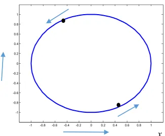
Figure 1 shows a circular orbit of a constant radius ρ0. Both stars are separated
by the distance l0=2ρ0. The angular position of the first star is defined by the phasor ψ1
( )
t =ρ0exp(
j tω0) ( )
;ϕ1 t =ω0t, and the second by( )
(
) ( )
2 t 0exp j t0 π ; 2 t 0t π
ψ =ρ ω + ϕ =ω + . This system is described by the equality
of two forces: the gravitational force of attraction and the centrifugal inertial force.
For the circular orbit of Figure 1 (no inspiral), the two forces are collinear and have opposite directions. They should have the same magnitude. This equality of forces is described by
2
2 0 0 2
0
4
g=Gmρ = c=mω ρ
F F . (1)
We get the following time-independent relations between the angular velocity ω0 and the radius ρ0:
3
0 2
0
4 Gm ρ
ω
= or 0 3
0
4 Gm ω
ρ
= . (2)
The orbital tangential velocity is v0=ω ρ0 0. Therefore, the kinetic energy of the system is 2
0 k
E =mv and the potential energy Ep= −2
ρ
0 Fg . The potential energy is negative. Its value equals twice the kinetic energy. Therefore, the total energy of the system is negative and time independent. Several authors derived formulae for calculation of the power of gravitational waves emitted by the sys-tem of Figure 1. The derivations apply linearized version of Einstein’s theory of relativity. Let us present two examples:Valeria Ferrari [2] derived the following formulae; 54 25 3
[ ]
032 W
5
G M
P
c l
µ
= ,
where m m1 2
M
µ = , M m m= 1+ 2 and l0=2ρ0 is the orbital separation. If
1 2
m m= , we get
[ ]
4 55 5 0
2 W
5 G m P
c ρ
= . (3)
In the book of Gasperini [3], we find 4 6
[ ]
0 232 W
5 G
P a
c ω
DOI: 10.4236/jmp.2018.910124 1956 Journal of Modern Physics
Figure 1. The circular orbit of binary stars. Cartesian coordinates (x, y).
the formula (2), we get again (3). The above presented well known theory does not explain the phenomenon of inspiral. The famous observations by Taylor and Hulse [4] [5] [6], of the binary pulsar PSR1913+16 have shown that the stars in-spiral. The instantaneous radius ρ(t) decrease and the instantaneous angular
ve-locityω
( )
t increase. In order to explain this phenomenon we introduced ade-scription of the circular system using the notion of instantaneous complex fre-quency [7] [8].
3. Instantaneous Complex Frequency Description of the
Circular Binary System
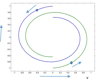
We have to show that due to the emission of gravitational waves, the trajectory of the stars is not circular since the instantaneous radius decrease in time and the angular velocity and tangential velocity increase in time. The stars are orbit-ing along spirals (Figure 2). A convenient method of description of this pheno-menon is the notion of instantaneous complex frequency. The phasor representing the first star has the form
( )
( )
( )
( )
( )
( )
1 0exp 0 d 0 ;
t
t s t t j s t t j t
ψ =ρ + ϕ =α + ω
∫
(4)and the second one
( )
( )
( )
2 0exp 0 d 0 π
t
t s t t j
ψ =ρ + ϕ +
∫
, (5)α
(t) is called instantaneous radial frequency and ω(t)—instantaneous angular frequency. The instantaneous radius is( )
0exp 0( )
dt
t t t
ρ =ρ α
∫
. In the-1 -0.8 -0.6 -0.4 -0.2 0 0.2 0.4 0.6 0.8 1 -1
-0.8 -0.6 -0.4 -0.2 0 0.2 0.4 0.6 0.8 1
DOI: 10.4236/jmp.2018.910124 1957 Journal of Modern Physics Figure 2. Inspiral orbits with enlarged rate of inspiral of binary stars. Cartesian coordi-nates (x, y).
simplest description of the properties of inspiral, the instantaneous complex frequency is time independent: s t
( )
= − +α0 jω0. In this case, the Cartesian coordinates of the orbit are:o For the first star x t
( )
=ρ0exp(
−α0t) ( )
cos ω0t ;( )
0exp(
0) ( )
sin 0y t =ρ −αt ωt ;
o For the second x t
( )
= −ρ0exp(
−α0t) ( )
cos ω0t ;( )
0exp(
0) ( )
sin 0y t = −ρ −α t ωt .
We have to explain why the stars accelerate by orbiting along the inspiral orbit. Let us show that the gravitational force 2
( )
24
g Gm
F
t
ρ
= and the centrifugal force
2 0
c c
F m= ω ρ differ by magnitude and direction. The orbital distance
( )
0 0( )
2ρ t =2 expρ − tα t td
∫
is a line connecting the mass centers through theorigin (0, 0) and defines the direction of gravitation force. Differently, the direc-tion of the centrifugal force Fc is defined by the curvature radius ρc. The
geome-try of the addition of the two forces is presented in Figure 3 (with large rate of inspiral). In the case α
( )
t = −α0, the angle γ is given by the formulae (see Ap-pendix 1)(
)
(
)
(
(
)
)
(
)
(
)
(
)
(
)
0 0 0
2
0 0 0
2 0 0
tan 0 , sin 0 ,
1 1
cos 0 .
1
t t
t
α α ω
γ γ
ω α ω
γ
α ω
−
= = − = =
+
= =
+
DOI: 10.4236/jmp.2018.910124 1958 Journal of Modern Physics
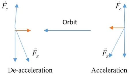
Figure 3. The gravitation force Fg is not collinear with the
centripetal force Fc the forces Fc and Fgcos
( )
γ canceland Fgsin
( )
γ has the direction of the tangent of the orbit causing de-acceleration (right) or deceleration (left).The inspiral orbit is defined by the equation
( )
Gravitational force cos×
γ
t =Centrifugal force. (7)However, there is a tangential force (see Figure 3)
( )
tan
Tangential force=F =Gravitational force sin×
γ
t . (8)However, for the quasi-circular orbit, the tangential force is extremely small. This force induces acceleration of the mass m given by
( )
tana t =mF . (9) In consequence, the instantaneous angular frequency is increasing in time
( )
0 0( )
d 2π( )
t
t a t t
T t
ω =ω +
∫
= (10)where T(t) is a decreasing instantaneous period. The energies of the system also increase in time. The instantaneous tangential velocity of the stars is
( )
( ) ( )
cv t =ω t ρ t . (11) The curvature radius is (see Appendix 2)
( )
(
(
)
)
(
)
0
3 2 2 0 0
0 2
0 0
1 e
1
t
c t α
α ω
ρ ρ
α ω
− +
=
− . (12)
The instantaneous kinetic energy of both stars is
( )
2( )
k
E t =mv t and the
instantaneous negative potential energy is
( )
( )
( )
24
p g Gm
E t F t
t
ρ
ρ
= = − . We start
the investigations with Equation (2). We can define the value of the radius ρ0 or
of ω0 but not of both. Our choice is the valueω0=2πT0=2.259554 10 rad s× -4
[
]
;[ ]
4 0 2.788720 10 s
T = × measured by Taylor and Hulse [8]. Using (2), we get the following values: the radius 8
[ ]
0 9.706500 10 m
ρ = × . The tangential velocity
equals 6
[
]
0 0 2.193236 10 m s
v=ω ρ = × (about 219 km/s). The kinetic energy of both stars is 2 1.346134 10 J41
[ ]
k
[image:5.595.262.490.72.200.2]DOI: 10.4236/jmp.2018.910124 1959 Journal of Modern Physics (magnitude twice of Ek) is Ep= −Gm2
(
2ρ0)
= −2.692268 10 J× 41[ ]
= −2Ek. Thetotal energy of the system is negative. The power of the gravitational waves emitted by the system given by Equation (3) is P=6.523698 10 W× 23
[ ]
.1) Estimation of the value of the radial frequency α0
The decrease of the radius of the circular model in one period T0 is
( 0 0)
0 0 2π
1 0e αT 0e α ω
ρ =ρ − =ρ − . (13)
We have an increase of the negative value of the potential energy
(
)
2
1 0 0
1 0
1 2π
4 4
p Gm Gm
E α ω
ρ ρ
= − ≈ − + . (14)
Therefore, we get the increase
(
)
1 0 0
0
2π 4
p Gm
E α ω
ρ −
∇ ≈ . (15)
Assuming arbitrary that this increase should be equal to the energy emitted by gravitational waves during one period we get
(
)
1 0 0 0 0
0
2π 2π
4
p Gm
E α ω PT P ω
ρ −
∇ ≈ = = . (16)
Therefore,
1 23 41 18
0 s 6.526980 10 2.692268 10 2.424343 10
p
P E
α ≈ − − = − × × = − × −
. (17)
2) The increase of the angular frequency (or decrease of the period T0)
during the inspiral
Taylor and Hulse have measured that the period of the PSR system decreases by 76.5 μs per year [6]. Let us derive a formula for this decrease for the circular system. We insert in Equation (2)
( )
00e t
t α
ρ =ρ − in place of ρ
0 getting
( )
0( )
00 3 3 2 2 0 0 3 4 0 e e 4 e t t t Gm
t α α T t T α
ω ω
ρ
− −
= = → = . (18)
The decrease of the period per year is
( )
32 0 year 6[ ]
year 0 year 0 1 e 32 0 0 year 3.18022 10 s
t
T T T t T − α T tα −
∇ = − = − ≈ − = ×
. (19)
It is more than one order of magnitude smaller in comparison to 76, 5 μs per year of the PSR system. Therefore, the circular model cannot be applied to de-scribe the properties of the PSR elliptical system.
3) The increase of the negative value of the potential energy The potential energy at the moment t = 0 is
( )
2 41[ ]
0
0 2.692268 10 J
2
p Gm
E
ρ
= − = − × . (20)
The value after one year is
( )
year 20 year[ ]
0
J 2 e
p t
Gm
E t α
ρ −
DOI: 10.4236/jmp.2018.910124 1960 Journal of Modern Physics The increase is
( )
0 e(
0 yeart 1)
2.052708 10 J31[ ]
p p
E E α
∇ = − = − × . (22)
The division by tyear yields the power
[ ]
23
year
6.526917 10 W
p
E P
t
∇
= = − × , (21)
i.e., exactly the value defined by Equation (3) which represents the power of the emitted gravitational waves. This result validates the correctness of Equation (17) defining α0 and Equation (19) defining the delay per year. The negative sign of
this power is applied in the book of Gasperini [3] with no comment. We found that the authors of reference [9] derived a formula with a negative sign of the gravitational “Poynting vector” also with no comment.
4) The inspiral time
The main goal of this paper is to validate the explanation of the nature of gravity presented in [1]. Having this in mind, let us describe only briefly the process of inspiral. During each period the radius
( )
0exp(
0( )
d)
t
t t t
ρ =ρ −
∫
α isa bit shorter, each next period is shorter corresponding to an increase of the an-gular frequency which is a function of time. As well, the instantaneous radial frequency increases with time. The angular frequency is
( )
( )
2 32 0( )
0 0
3 e ;
4
t
Gm
t t
t
α
ω ω α α
ρ
= = = . (22)
We get
( )
32 0 0et
T t =T − α and
( )
( )
32 00 0 0 0
3 1 e
2
t
T t T T t T − α − T tα
∇ = − = − ≈
. (23)
The instantaneous radius is
( )
( )
0( )
0exp 0 d 0e ; 0
t t
t t t α t
ρ =ρ − α ≈ρ − α ≈α
∫
. (24)The decrease of the radius during a year is
(
0 year)
year 0 1 e t α
ρ ρ −
∇ = − . (25)
The overestimated number of years of the total inspiral (overestimated since calculated using the constant value α0) is
[
]
0 year
10 0
year 0 year
1 ~ 1
Number of years 1.098 10 years
1 e αt t
ρ
ρ − α
= = ≈ = ×
∇ − . (27)
5) Concluding remarks about the circular system
During a single revolution, the emitted power may be classified as time inde-pendent since the increase is negligible. The directional pattern
( )
[
W steradian]
fre-DOI: 10.4236/jmp.2018.910124 1961 Journal of Modern Physics quency with a circular polarization [2]. In long times, there is an increase of the power and the negative energy of the system. Therefore, assuming that the gra-vitational waves carry positive energy, the emission is at the cost of increasing negative energy of the system. The presented theory of inspiral is valid only in the frame of a linear gravitation. The phenomena in the last stage of inspiral are certainly governed by nonlinear effects. Recently, the LIGO system registered a chirp like signal of duration about 0.17 [s] emitted by two black holes shortly before the collapse [10] [11]. Certainly, a linear theory is unable to describe this signal.
4. The Theoretical Model of the Binary Pulsar PSRB1913+16
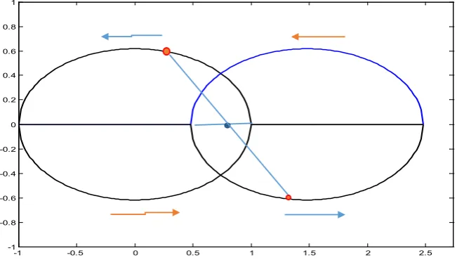
The PSR system differs considerably from the above described circular system. The two stars are orbiting along elliptical orbits (see Figure 4) around a com-mon center of mass located in the focus. We consider again equal masses
1 2
m m= =m. The data of this system measured by Taylor and Hulse are pre-sented in Appendix 1. In the circular model, the distance between the stars, the angular velocity ω, the tangential velocity and the potential and kinetic energies could be classified as constant during a single orbital time. This is not the case in the PSR system. For example, the velocity changes from vmax = 450 [km/s] to 120
[km/s]. These changes overshadow by several orders the inspiral change due to the emission of gravitational waves.
1) The description of the elliptical orbits in polar coordinates centered at the focus
The elliptical orbit of the first star can be defined in polar coordinates (ρ, φ) centered at the right focus of the left ellipse (Figure 4). The radius ρ in terms of the angle φ is given by the formula
( )
1 2( )
1 cos
a ε
ρ ϕ
ε ϕ
− =
+ (28)
and for the second one centered in the left focus of the right ellipse is
( )
1(
2)
1 cos π
a ε
ρ ϕ
ε ϕ
− =
− + (29)
Note that the angle φ is a function of time. However, our derivations have the form of functions of φ. The inverse function t(φ) has no closed form. Our goals do not require the presentation of these relations.
For φ = 0, we get periastrone separation =2 1a
[
−ε]
and for ϕ = π, theapa-strone separation =2 1a
[
+ε]
. The insertion of the semi-major axis[ ]
8
9.7506 10 m
a= × and eccentricity ε =0.617733 yields (see [6]):
[ ]
8Periastron separation 7.45466 10 m= × and
[ ]
8
Apastron separation 3.154477 10 m= × . 2) Why the stars accelerate and decelerate?
DOI: 10.4236/jmp.2018.910124 1962 Journal of Modern Physics Figure 4. The elliptical orbits of the PSR system. The stars (red points) rotate anti clock. Blue arrows: deceleration. Red arrows: acceleration.
case of the two elliptical orbits we have large accelerations and decelerations during each period. Again, the gravitational attraction force is given by
( )
2( )
2[ ]
N 4g ϕ = Gmρ ϕ
F (30)
and the centrifugal force is given by
( )
2( ) ( )
[ ]
Nc t =mω ϕ ρ ϕc
F (31)
where ρc is the curvature radius of the ellipse and the angular velocity is defined
by the rotation of the curvature radius. Again, the force vectors have different direction defined by the angle γ. The gravitational force can be represented by a vector sum of two perpendicular terms (Figure 3). The term
( ) ( )
cos 4 2( )
2 cos( )
[ ]
Ng ϕ γ = ρ ϕGm γ
F (32)
has the direction of (30) perpendicular to the tangent of the ellipse and the term
( ) ( )
sin 2( ) ( )
2 sin[ ]
N4
g ϕ γ = ρ ϕGm γ
F (33)
represents a tangential force. Equating the terms (31) and (32) yields the follow-ing formula for the local angular velocity (local means the function of ϕ).
( )
( ) ( )
cos( )
[
rad s]
4 c
Gm γ
ω ϕ
ρ ϕ ρ ϕ
= . (34)
The local tangential acceleration is
( )
( ) ( )
( ) ( )
22
sin sin m s
4
g Gm
a ϕ ϕ γ m γ
ρ ϕ
=F = . (35)
The local velocity of the stars by orbiting from periastrone to apastron is (de-celeration)
-1 -0.5 0 0.5 1 1.5 2 2.5
-1 -0.8 -0.6 -0.4 -0.2 0 0.2 0.4 0.6 0.8 1
DOI: 10.4236/jmp.2018.910124 1963 Journal of Modern Physics
( )
π( )
max 0 d
v ϕ =v −
∫
a ϕ ϕ (36)and in opposite direction (acceleration)
( )
2π( )
min π d
v ϕ =v +
∫
a ϕ ϕ. (37)The mean velocity (in terms of φ) is the same for both directions
( )
π mean 1π 0 d
v =
∫
v ϕ ϕ. (38)The local tangential velocity is alternatively defined as
( )
( ) ( )
cv ϕ =ω ϕ ρ ϕ (39)
Where ρc is the local curvature radius (see Figure 5). The local velocity is shown
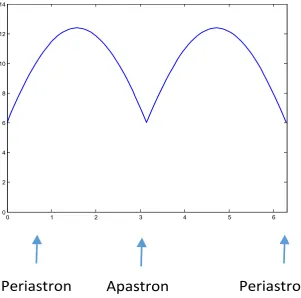
in Figure 6. The maximum value equals 448.172 [km/s] and the minimum 106.287 (compare with Appendix 1).
Note that in this model, the maxima and minima of the velocity are located near the periastrone and apastrone (not exactly at these locations). The mean value in terms of φ (as in Equation (38)) is 269.782 [km/s]. The time average is
( )
circumference of ellipse 181.757 km s[
]
time of a single revolutionv t = = . (40)
[image:10.595.217.519.409.707.2]The local average differs from the time average by the factor 1.319. The local angular velocity is shown in Figure 7.
Figure 5. Curvature radius in terms of φ.Vertical scale × 108.
0 1 2 3 4 5 6
0 2 4 6 8 10 12 14
DOI: 10.4236/jmp.2018.910124 1964 Journal of Modern Physics
Figure 6. Orbital velocity [km/s] in terms of φ. Note the localization of vmax not at
perias-tron.
Figure 7. Angular velocity ω (rad/s) in terms φ. Vertical scale 10−8.
3) Kinetic and potential energies in the PSR system The local kinetic energy is (Figure 8)
( )
2( )[ ]
Jk
E ϕ =mv ϕ (41)
0 1 2 3 4 5 6
0 50 100 150 200 250 300 350 400 450 500
0 1 2 3 4 5 6
[image:11.595.209.537.370.655.2]DOI: 10.4236/jmp.2018.910124 1965 Journal of Modern Physics
Figure 8. Kinetic energy (upper curve at φ = π) and themagnitude ofpotential energy in
terms ofφ. Vertical scale ×1041.
and the local negative potential energy is
( )
( )
2[ ]
J 2P Gm
E ϕ
ρ ϕ −
= . (42)
The corresponding local averages are 2.38257 10 J41
[ ]
k
E = × and
[ ]
414.369225 10 J
p
E = − × . The ratio is Ep Ek =2.02435 2≈ , i.e., almost the
value defined by the circular system. It is reasonable to assume that the same ra-tio is valid for time averages.
4) Concluding remarks about the PSR system
Differently to the circular system the power emitted during a single revolution is a function of time and the radiation pattern σ Ω
( )
[
W steradian]
is a period-ic function of time. Therefore, the reported by Taylor and Hulse power of the emitted gravitational waves P = 7.35 × 1024 [W] should be classified as a meanvalue.
5. Final Conclusions
o Both orbits, the circular and the elliptical, are defined by two forces of oppo-site directions: the centrifugal force and a term of the gravitational force (see Figure 3). It is logical to assume that both forces have the same physical ex-planation: the anisotropic energy exchange as described in reference [1]. Here, both anisotropies of radiation cancel. The other part of the gravitation-al force responsible for tangentigravitation-al acceleration or deceleration is the result of the tangential anisotropy of radiation.
0 1 2 3 4 5 6
DOI: 10.4236/jmp.2018.910124 1966 Journal of Modern Physics o In the case of a circular orbit, the tangential acceleration is extremely small.
We have shown that the notion of the instantaneous complex frequency is a convenient tool to study the process of inspiral of circular systems in the range of a linear gravitational force.
Arguments in favor of the radiation recoil nature of gravity presented in [1 m]
In 2015, the author presented a paper “Gravitational Forces Explained as the Result of Exchange between Baryonic Matter and the Quantum Vacuum” [1]. Let us present arguments in favor of this theory in terms of the description of orbiting double stars given in this paper:
o The orbit is defined by two forces: the gravitational force directed towards inside of the orbit and the centrifugal force directed towards the outside of the orbit. The forces are not collinear.
o The centripetal force is perpendicular to the tangent of the orbit.
o The gravitational force except some points is not perpendicular to the tan-gent and can be decomposed in two terms: the perpendicular compensates the centripetal force. The two forces cancel.
o The tangent force is responsible for acceleration or deceleration of the star. o In the case of the common nearly circular orbit of the stars, we have an
ex-tremely small acceleration. In the case of a double-elliptical orbit, we have large accelerations and deceleration.
o The cancelation of the two forces shows that gravity and inertia have the same physical origin. They are recoil forces of radiation. The radiation tern should be symmetric w.r.t. the tangent of the orbit. Differently, the pat-tern is asymmetric w.r.t. the line perpendicular to the orbit resulting in a re-coil force of radiation.
In a word, it is logical to assume that all described here forces are recoil forces of radiation. The radiation pattern is symmetric w.r.t. the tangent of the orbit (cancellation of gravitation and inertia) and asymmetric w.r.t. the line perpen-dicular to the orbit, i.e., the direction of the curvature radius.
Conflicts of Interest
The authors declare no conflicts of interest regarding the publication of this pa-per.
References
[1] Hahn, S.L. (2015) Journal of Modern Physics, 6,1135-1145. https://doi.org/10.4236/jmp.2015.68117
[2] Ferrari, V. (2010) The Quadrupole Formalism Applied to Binary Systems. https://www.-ego-gw.it/public/events/vesf
[3] Gasperini, M. (2017) Theory of Gravitational Interactions. 2nd Edition, Springer. [4] Press Release (1993) About the Nobel Prize in Physics, Royal Swedish Academy of
DOI: 10.4236/jmp.2018.910124 1967 Journal of Modern Physics [5] The Binary Pulsar PSR1913+16.
http://www.astrocornell.edu/academics/PSR1913+16
[6] Johnstone, R. http://www.johnstonsarchive.net./relativity/binarypulsar.html [7] Hahn, S. (1939) The Instantaneous Complex Frequency Concept and Its
Applica-tion in the Analysis of Building up OscillaApplica-tions in Oscillator. Proceedings of Vibra-tions Problems, No. 1, 29-46.
[8] Hahn, S.L. and Snopek, K.M. (2016) Complex and Hypercomplex Analytic Signals. Theory and Applications, Artech House, Boston-Landon.
[9] Mironov, V.L. and Mironov, S.V. (2014) Journal of Modern Physics, 5, 917-929. https://doi.org/10.4236/jmp.2014.510095
DOI: 10.4236/jmp.2018.910124 1968 Journal of Modern Physics
Appendix 1
This paper is illustrated by the properties of the binary pulsar PSR1913+16, a system of two binary neutron stars discovered and measured during many years by Taylor and Hulse [7] [8]. This great achievement of radioastronomy and also of time-frequency metrology was awarded by the Nobel Prize in physics in 1993. Let us repeat here the data compiled by Robert Johnston [8].
Mass of detected pulsar 30
[ ]
1 1.441 solar mass 2.8764 10 kg
m = × = × and of its
companion 30
[ ]
2 1.387 s.m. 2.7205 10 kg
m = × = × .
Orbital period T0 =7.7511939106 hr
[ ]
=27807.19557 s[ ]
. Eccentricity of the elliptical orbits ε =0.617131.Semi-major axis 2a=1950100 km
[ ]
(remark of this author: the name semi-major axis should be replaced by major axis. Semi-major axis is equal not 2a but a. Periastron separation 746600 km=[ ]
,[ ]
Apastron separation 3153600 km=Orbital velocity of stars relative to the center of mass: at periastrone 450 [km/s], at apastrone: 110 [km/s].
Appendix 2: The Derivation of the Curvature Radius of the
in Spiral Orbit
Let us define the in spiral orbit by the equation
( )
0e 0( )
dt
t s t t
ψ =ρ
∫
(A1)( )
(
) (
0)
s t = − α+ ∆ ∗ +α t j ω + ∆ ∗ω t (A2)
We assume that the binary stars have equal mass and rotate synchronously around common center of mass located at x = y = 0. The Cartesian coordinates of the first star are defined by the complex function ψ
( )
t =x t( )
+ jy t( )
with( )
(
0.5 2)
(
2)
0e cos 0 0.5
t t
x t =ρ −α+ ∆ ∗α ωt+ ∆ ∗ω t (A3)
( )
(
0.5 2)
(
2)
0e sin 0 0.5
t t
y t =ρ −α+ ∆ ∗α ωt+ ∆ ∗ω t (A4)
and for the second star
( )
(
0.5 2)
(
2)
0e cos 0 0.5
t t
x t = −ρ −α+ ∆ ∗α ω t+ ∆ ∗ω t (A5)
( )
(
0.5 2)
(
2)
0e sin 0 0.5
t t
y t = −ρ −α+ ∆ ∗α ωt+ ∆ ∗ω t (A6) The curvature radius at the point defined by t = t0 is
( )
(
)
(
( )
)
( ) ( ) ( ) ( )
2 2
0 0
0 0 0 0
c
x t y t y t x t x t y t
ρ
+
=
+
(A7)
Let us calculate the derivatives beginning with zero values of ∆α and ∆ω. We
have
( )
0( )
0( )
0 0e tcos 0 0e tsin 0
x t =
ρ
−α
−αω
t −ω
−αω
t
DOI: 10.4236/jmp.2018.910124 1969 Journal of Modern Physics
( )
0( )
0( )
0 0e tsin 0 e t 0cos 0
y t =
ρ
−α
−αω
t + −αω
ω
t
(A9)
( )
( )
( )
( )
( )
0
0 2
0 0 0 0 0 0
2
0 0 0 0 0
e cos e sin e sin e cos
t t
t t
x t t t
t t
α α
α α
ρ α
ω
α ω
ω
α ω
ω
ω
ω
− − − − = + + −
( )
( )
( )
( )
( )
0 0 0 20 0 0 0 0 0
2
0 0 0 0 0
e sin e cos e cos e sin
t t
t t
y t R t t
t t
α α
α α
α
ω
α ω
ω
α ω
ω
ω
ω
− − − − = − − −
The insertion using t = 0 yields
( )
(
(
)
)
(
(
)
)
(
)
0 0 3 3 2 22 2 2
0 0
0 0
0 2 2 0 2
0 0
0 0 0
1
e e
1
t t
c t α α
α ω
α ω
ρ ρ ρ
α ω
ω ω α
− + − +
= =
−
− (A10)
Of course, for a circular orbit α0 = 0 and ρc = ρ0. Otherwise, ρc > ρ0. The center
of the curvature radius is located at
( ) ( )
(
( ) ( ) ( ) ( )
(
( )
)
)
(
( )
)
( ) ( )
(
( ) ( ) ( ) ( )
(
( )
)
)
(
( )
)
2 2
0 0
0 0
0 0 0 0
2 2
0 0
0 0
0 0 0 0
;
.
c
c
x t y t
x x t y t
y t x t y t x t
x t y t
y y t x t
y t x t y t x t
+ = − − + = + − (A11)
If t=0, x
( )
0 =ρ0, y( )
0 =0, x( )
0 = −α ρ0 0, y( )
0 =ω ρ0 0,( )
(
2 2)
0 0 0
0
x =
ρ α
−ω
, y
( )
0 = −2α ω0 0 0R . The insertion yields( )
( )
00 0
0 0, 0
c c
x y α ρ
ω
= = − . The angle between ρ0 and
c
ρ is
(
)
(
)
(
(
)
)
(
)
(
)
(
)
(
)
0 0 0
2
0 0 0
2 0 0
tan 0 , sin 0 ,
1 1 cos 0 1 t t t
α α ω
ϕ ϕ
ω α ω
ϕ α ω = = − = = + = = +
The curvature radius of an ellipse in Cartesian coordinates (x, y) is 3
2 2 2
2 2
4 4
c a b ax by
![Figure 6. Orbital velocity [km/s] in terms of φ. Note the localization of vmax not at perias-tron](https://thumb-us.123doks.com/thumbv2/123dok_us/9267342.417311/11.595.209.537.370.655/figure-orbital-velocity-terms-note-localization-vmax-perias.webp)

