arXiv:0803.4323v1 [hep-th] 31 Mar 2008
Preprint typeset in JHEP style - HYPER VERSION ITP-UU-08-15
SPIN-08-14
TCDMATH 08-03
The S-matrix of String Bound States
Gleb Arutyunova∗ † and Sergey Frolovb†
a Institute for Theoretical Physics and Spinoza Institute,
Utrecht University, 3508 TD Utrecht, The Netherlands
b School of Mathematics, Trinity College, Dublin 2, Ireland
Abstract: We find the S-matrix which describes the scattering of two-particle
bound states of the light-cone string sigma model on AdS5 ×S5. We realize the
M-particle bound state representation of the centrally extended su(2|2) algebra on the space of homogeneous (super)symmetric polynomials of degree M depending on two bosonic and two fermionic variables. The scattering matrix SM N of M- and
N-particle bound states is a differential operator of degree M +N acting on the product of the corresponding polynomials. We require this operator to obey the invariance condition and the Yang-Baxter equation, and we determine it for the two cases M = 1, N = 2 and M = N = 2. We show that the S-matrices found sat-isfy generalized physical unitarity, CPT invariance, parity transformation rule and crossing symmetry. Although the dressing factor as a function of four parameters
x+1, x−1, x+2, x−2 is universal for scattering of any bound states, it obeys a crossing symmetry equation which depends onM and N.
∗Email: G.Arutyunov@phys.uu.nl, frolovs@maths.tcd.ie
Contents
1. Introduction and summary 2
2. Bound state representations 7
2.1 Centrally extended su(2|2) algebra 8
2.2 The atypical totally symmetric representation 9
2.3 The rapidity torus 12
3. S-matrix in the superspace 13
3.1 Operator realization ofsu(2|2)C 13
3.2 S-matrix operator 15
3.3 Matrix form of the S-matrix 19
3.4 General properties of S-matrix 20
4. S-matrices 27
4.1 The S-matrix SAA 27
4.2 The S-matrix SAB 32
4.3 The S-matrix SBB 33
5. Crossing symmetry 37
5.1 String S-matrix 37
5.2 Crossing symmetry equations for the S-matrices 40
6. Appendices 45
6.1 The S-matrix SAB 45
6.1.1 Invariant differential operators for SAB 45
6.1.2 Coefficients of SAB 47
6.1.3 Matrix form of invariant differential operators Λk 48
6.2 The S-matrix SBB 50
6.2.1 Invariant differential operators for SBB 50
6.2.2 Coefficients of the S-matrix SBB 53
1. Introduction and summary
It has been recognized in recent years that the S-matrix approach provides a powerful tool to study the spectra of both the AdS5×S5 superstring and the dual gauge theory
[1]-[8]. In the physical (light-cone) gauge the Green-Schwarz string sigma-model [9] is equivalent to a non-trivial massive integrable model of eight bosons and eight fermions [10, 11]. The corresponding scattering matrix, which arises in the infinite-volume limit, is determined by global symmetries almost uniquely [8, 12], up to an overall dressing phase [4] and the choice of a representation basis. A functional form of the dressing phase in terms of local conserved charges has been bootstrapped [4] from the knowledge of the classical finite-gap solutions [13]. Combining this form with the crossing symmetry requirement [14], one is able to find an exact, i.e. non-perturbative in the coupling constant, solution for the dressing phase [15] which exhibits remarkable interpolation properties from strong to weak coupling [16]. The leading finite-size corrections to the infinite-volume spectrum are encoded into a set of asymptotic Bethe Ansatz equations [6] based on this S-matrix.
In more detail, a residual symmetry algebra of the light-cone Hamiltonian H
factorizes into two copies of the superalgebrasu(2|2) centrally extended by two cen-tral charges, the latter depend on the operatorPof the world-sheet momentum [17]. Correspondingly, the S-matrix factorizes into a product of two S-matrices SAA, each of them scatters two fundamental supermultiplets A. Up to a phase, the S-matrix
SAA is determined from the invariance condition which schematically reads as
SAA·J12 =J21·SAA,
where J12 is a symmetry generator in the two-particle representation.
As in some quantum integrable models, it turns out that, in addition to the supermultiplet of fundamental particles, the string sigma-model contains an infinite number of bound states [18]. They manifest themselves as poles of the multi-particle S-matrix built over SAA. The representation corresponding to a bound state of M
fundamental particles constitutes a short 4M- dimensional multiplet of the centrally extended su(2|2) algebra [19, 20]. It can be obtained from theM-fold tensor product of the fundamental multiplets by projecting it on the totally symmetric component. A complete handle on the string asymptotic spectrum and the associated Bethe equations requires, therefore, the knowledge of the S-matrices which describe the scattering of bound states. This is also a demanding problem for understanding the finite-size string spectrum within the TBA approach [21].
A well-known way to obtain the S-matrices in higher representations from a fundamental S-matrix is to use the fusion procedure [22]. A starting point is a multi-particle S-matrix
where the (complex) momentap1, . . . , pM provide a solution of theM-particle bound state equation and the indexa denotes an auxiliary space being another copy of the fundamental irrep. Next, one symmetrises the indices associated to the matrix spaces 1, . . . , M according to the Young pattern of a desired representation. The resulting object must give (up to normalization) an S-matrix for scattering of fundamental particles with M-particle bound states. A proof of the last statement uses the fact that at a pole the residue of the S-matrix is degenerate and it coincides with a pro-jector on a (anti-)symmetric irrep corresponding to the two-particle bound state. This is, e.g., what happens for the rational S/R-matrices based on the gl(n|m) su-peralgebras. The fusion procedure for the corresponding transfer-matrices and the associated Baxter equations have been recently worked out in [23, 24].
The fundamental S-matrixSAA behaves, however, differently and this difference can be traced back to the representation theory of the centrally extended su(2|2). LetVA be a four-dimensional fundamental multiplet. It characterizes by the values
of the central charges which are all functions of the particle momentum p. For the generic values of p1 and p2 the tensor product VA(p1)⊗VA(p2) is an irreducible
long multiplet [8, 19]. In the special case when momenta p1 and p2 satisfy the
two-particle bound state equation the long multiplet becomes reducible. With the proper normalization of the S-matrix the invariant subspace coincides with the null space
SAA(p1, p2)Vker = 0, Vker⊂VA⊗VA.
Indeed, ifv ∈Vker, thenJ12v ∈Vkerdue to the intertwining property of the S-matrix: SAA·J12v =J21·SAAv = 0. Being reducible at the bound state point, the multiplet VA⊗V Ais, however,indecomposable. In particular, there is no invariant projector on either Vker or on its orthogonal completion. The bound state representation we are
interested in corresponds to a factor representation on the quotient space VA/Vker.
In this respect, it is not clear how to generalize the known fusion procedure to the present case.1
The absence of apparent fusion rules motivates us to search for other ways to determine the scattering matrices of bound states. An obvious suggestion would be to follow the same invariance argument for the bound state S-matrices as for the fundamental S-matrix together with the requirement of factorized scattering, the latter being equivalent to the Yang-Baxter (YB) equations. A serious technical problem of this approach is, however, that the dimension of the M-particle bound state representation grows as 4M, so that the S-matrixSM N for scattering of theM -and N-particle bound states will have rank 16MN. Even for small values ofM and
N working with such big matrices becomes prohibitory complicated. Although, we are ultimately interested not in the S-matrices themselves but rather in eigenvalues
1
The usual fusion procedure works, however, for the rank one sectors ofSAA, in which case it
of the associated transfer-matrices, we fist have to make sure that the corresponding scattering matrices do exist and they satisfy the expected properties.
The aim of this paper is to develop a new operator approach to deal with the bound state representations. This approach provides an efficient tool to solve both the invariance conditions and the YB equations and, therefore, to determine the S-matrices SM N, at least for sufficiently low values of M and N.
Our construction relies on the observation that theM-particle bound state rep-resentation VM of the centrally extended su(2|2) algebra can be realized on the
space of homogeneous (super)symmetric polynomials of degree M depending on two bosonic and two fermionic variables, wa and θα, respectively. Thus, the representa-tion space is identical to an irreducible short superfield ΦM(w, θ). In this realization the algebra generators are represented by linear differential operators J in wa and
θα with coefficients depending on the representation parameters (the particle mo-menta). More generally, we will introduce a space DM dual to VM, which can be
realized as the space of differential operators preserving the homogeneous gradation of ΦM(w, θ). The S-matrix SM N is then defined as an element of
End(VM ⊗VN)≈V M ⊗VN ⊗DM ⊗DN.
On the product of two superfields ΦM(w1, θ1)ΦN(w2, θ2) it acts as a differential op-erator of degreeM+N. We require this operator to obey the following intertwining property
SM N·J12 =J21·SM N,
which is the same invariance condition as before but now implemented for the bound state representations. For two su(2) subgroups of su(2|2) this condition literally means the invariance of the S-matrix, while for the supersymmetry generators it involves the brading (non-local) factors to be discussed in the main body of the paper. Thus, the S-matrix is an su(2)⊕su(2)-invariant element of End(VM ⊗VN)
and it can be expanded over a basis of invariant differential operators Λk:
SM N =X k
akΛk.
As we will show, it is fairly easy to classify the differential su(2)⊕su(2) invariants Λk. The coefficients ak are then partially determined from the remaining invariance conditions with the supersymmetry generators. It turns out, however, that if the tensor product VM ⊗VN has m irreducible components then m−1 coefficients a
computational time, therefore, we give it a preference in comparison to the matrix approach.
Having established a general framework, we will apply it to construct explic-itly the operators SAB and SBB, which are the S-matrices for scattering processes involving the fundamental multiplet A and a multiplet B corresponding to the two-particle bound state. We will show thatSAB is expanded over a basis of 19 invariant differential operators Λk and all the corresponding coefficients ak up to an overall normalization are determined from the invariance condition. Construction of SBB
involves 48 operators Λk. This time, two of ak’s remain undetermined by the in-variance condition, one of them corresponding to an overall scale. As to the second coefficient, we find it by solving the YB equations. It is remarkable that with one coefficient we managed to satisfy two YB equations: One involving SAB and SBB, and the second involving SBB only. This gives an affirmative answer to the question about the existence of the scattering matrices for bound states.
Recall that the universal cover of the parameter space describing the fundamental representation of the centrally extended su(2|2) is an elliptic curve (a generalized rapidity torus with real and imaginary periods 2ω1 and 2ω2, respectively) [14]. Since
the particle energy and momentum are elliptic functions with the modular parameter
−4g2, whereg is the coupling constant, the fundamental S-matrixSAAcan be viewed as a function of two variablesz1 andz2 with values in the elliptic curve. Analogously,
theM-particle bound state representation can be uniformized by an elliptic curve but with another modular parameter −4g2/M2. Correspondingly, in generalSM N(z
1, z2)
is a function on a product of two tori with differentmodular parameters.
In a physical theory, in addition to the YB equation, the operatorsSmust satisfy a number of important analytic properties. RegardingS as a function of generalized rapidity variables, we list them below.
• Generalized Physical Unitarity
S(z1∗, z2∗)†·S(z1, z2) =I • CPT Invariance
S(z1, z2) T
=S(z1, z2)
• Parity Transformation Rule
S−1(z1, z2) =S(−z1,−z2)
P
• Crossing Symmetry
the S-matrixSM N without appealing to the YB equations. Concerning the universal R-matrix, would it exist, one could use it to deduce all the bound states S-matrices
SM N and the fusion procedure would not be required. Due to non-invertibility of the Cartan matrix for su(2|2), existence of the universal R-matrix remains an open problem. On the other hand, at the classical level [32] one is able to identify a universal analogue of the classical r-matrix [33, 34]. It is of interest to verify if the semi-classical limit of our S-matrices agrees with this universal classicalr-matrix [35].
As was explained in [21], to develop the TBA approach for AdS5×S5 superstring
one has to find the scattering matrices for bound states of the accompanying mirror theory. The bound states of this theory are “mirrors” of those for the original string model. Moreover, the scattering matrix of the fundamental mirror particles is obtained from SAA by the double Wick rotation. The same rotation must also relate the S-matrices of the string and mirror bound states, which on the rapidity tori should correspond to shifts by the imaginary quarter-periods.
The leading finite-size corrections [36]-[38] to the dispersion relation for fun-damental particles (giant magnons [39]) and bound states can be also derived by applying the perturbative L¨uscher approach [40], which requires the knowledge of the fundamental S-matrix [41]-[45]. It is quite interesting to understand the meaning of the bound state S-matrices in the L¨uscher approach and use them, e.g., to compute the corrections to the dispersion relations corresponding to string bound states.
Let us mention that our new S-matrices might also have an interesting physical interpretation outside the framework of string theory and the AdS/CFT correspon-dence [46]. Up to normalization, SAA coincides [19, 25] with the Shastry R-matrix [47] for the one-dimensional Hubbard model. The operators SAB and SBB might have a similar meaning for higher Hubbard-like models describing the coupling of the Hubbard electrons to matter fields. Also, the representation of the S-matrices in the space of symmetric polynomials we found provides a convenient starting point for a search of possible q-deformations [48]. The space of symmetric polynomials admits a natural q-deformation with the corresponding symmetry algebra realized by difference operators. It would be interesting to find the q-deformed versions of
SAB and SBB along these lines.
2. Bound state representations
In this section we discuss the atypical totally symmetric representations of the cen-trally extended su(2|2) algebra which are necessary to describe bound states of the light-cone string theory on AdS5×S5. These representations are 2M|2M-dimensional,
2.1 Centrally extended su(2|2) algebra
The centrally extendedsu(2|2) algebra which we will denote su(2|2)C was introduced
in [8]. It is generated by the bosonic rotation generators Lab, Rαβ, the supersym-metry generators Qαa, Q†aα, and three central elements H, C and C† subject to the following relations
Lab,Jc=δbcJa− 1 2δ
b aJc,
Rαβ,Jγ=δγβJα− 1 2δ
β αJγ,
Lab,Jc=−δc aJb+
1 2δ
b aJc,
Rαβ,Jγ =−δγ αJβ+
1 2δ
β αJγ,
{Qαa,Q†bβ}=δbaRαβ +δαβLba+1 2δ
a bδαβH,
{Qαa,Qβb}=ǫαβǫab C, {Q†aα,Q†bβ}=ǫabǫαβ C†. (2.1) Here the first two lines show how the indices c and γ of any Lie algebra generator transform under the action ofLab andRαβ. For the AdS5×S5 string model the central
elementHis hermitian and is identified with the world-sheet light-cone Hamiltonian, and the supersymmetry generators Qαa and Q†aα. The central elements C and C†
are hermitian conjugate to each other: (Qαa)†=Q†aα. It was shown in [17] that the central elements C and C† are expressed through the world-sheet momentum P as follows
C= i 2g(e
iP−1)e2iξ, C†=
−2ig(e−iP−1)e−2iξ, g =
√
λ
2π . (2.2)
The phase ξ is an arbitrary function of the central elements. It reflects an external U(1) automorphism of the algebra (2.1): Q → eiξQ, C → e2iξC. In our paper [12] the choice ξ= 0 has been made in order to match with the gauge theory spin chain convention by [8] and to facilitate a comparison with the perturbative string theory computation of the S-matrix performed in [49]. We use the same choice of ξ in the present paper too.
Without imposing the hermiticity conditions on the generators of the algebra the U(1) automorphism of the algebra can be extended to the external sl(2) auto-morphism [19], which acts on the supersymmetry generators as follows
e
Qαa=u1Qαa+u2ǫacQ†cγǫγα, Qe†aα=v1Q†aα+v2ǫαβQβbǫba,
Qαa =v1Qeαa−u2ǫacQe†cγǫγα, Q†aα =u1Qe†aα−v2ǫαβQeβbǫba,
(2.3)
where the coefficients may depend on the central charges and must satisfy the sl(2) condition
u1v1−u2v2 = 1.
Then, by using the commutation relations (2.1), we find that the transformed gen-erators satisfy the same relations (2.1) with the following new central charges
e
H= (1 + 2u2v2)H−2u1v2C−2u2v1C†,
e
C=u21C+u22C†−u1u2H, Ce†=v12C†+v22C−v1v2H.
If we now require that the new central chargesCe andCe†vanish, while the transformed supercharges Qe and Qe† are hermitian conjugate to each other, we find
u1 =v1 =
1
√
2
s
1 + √ H
H2−4CC†,
u2 =
C √
H2 −4CC†
1
u1
, v2 =
C† √
H2−4CC†
1
v1
.
(2.5)
With this choice of the parameters ui, vi, the new Hamiltonian takes the following simple form
e
H=pH2−4CC†.
We see that any irreducible representation of the centrally-extended algebra with
e
H6= 0 can be obtained from a representation of the usual su(2|2) algebra with zero central charges C = C† = 0. This will play an important role in our derivation of
the bound state scattering matrices.
2.2 The atypical totally symmetric representation
The atypical totally symmetric representation4ofsu(2|2)
Cwhich describesM-particle
bound states of the light-cone string theory on AdS5×S5 has dimension 2M|2M and
it can be realized on the graded vector space with the following basis
• a tensor symmetric in ai: |ea1...aMi, where ai = 1,2 are bosonic indices which
gives M + 1 bosonic states
• a symmetric in ai and skew-symmetric in αi: |ea1...aM−2α1α2i, where αi = 3,4 are fermionic indices which gives M −1 bosonic states. The total number of bosonic states is 2M.
• a tensor symmetric inai : |ea1...aM−1αi which gives 2M fermionic states.
We denote the corresponding vector space as VM(p, ζ) (or just VM if the values of
p and ζ are not important), where ζ = e2iξ. For non-unitary representations the parameters p and ζ are arbitrary complex numbers which parameterize the values of the central elements (charges) on this representation: H|eii = H|eii, C|eii =
C|eii, C†|eii = C|eii, where |eii stands for any of the basis vectors. The bosonic generators act in the space in the canonical way
Lab|ec1c2···cMi=δ
b
c1|eac2···cMi+δ
b
c2|ec1ac3···cMi+· · · −
M 2 δ
b
a|ec1c2···cMi Lab|ec1···cM−2γ1γ2i=δ
b
c1|eac2···cM−2γ1γ2i+δ
b
c2|ec1ac3···cM−2γ1γ2i+· · · − M−2
2 δ b
a|ec1···cM−2γ1γ2i
Lab|ec1c2···cM−1γi=δ b
c1|eac2···cM−1γi+δ
b
c2|ec1ac3···cM−1γi+· · · −
M −1 2 δ
b
a|ec1···cM−1γi, 4
and similar formulas for Rαβ
Rαβ|ec1c2···cMi= 0 Rαβ|ec1c2···cM−2γ1γ2i=δ
β
γ1|ec1···cM−2αγ2i+δ
β
γ2|ec1···cM−2γ1αi −δ
β
α|ec1···cM−2γ1γ2i
Rαβ|ec1c2···cM−1γi=δ
β
γ|ec1···cM−1αi −
1 2δ
β
α|ec1···cM−1γi.
Then the most general action of supersymmetry generators compatible with thesu(2) symmetry is of the form
Qαa|ec1c2···cMi=a1 δ
a
c1|ec2···cMαi+δ
a
c2|ec1···cMαi+· · ·
,
Qαa|ec1c2···cM−2γ1γ2i=b2ǫ
acM−1 ǫ
αγ1|ec1···cM−1γ2i −ǫαγ2|ec1···cM−1γ1i
,
Qαa|ec1c2···cM−1γi=b1ǫ
acMǫ
αγ|ec1···cMi+a2 δ
a
c1|ec2···cM−1αγi+δ
a
c2|ec1···cM−1αγi+· · ·
,
where the constants a1, a2, b1, b2 are functions of g, p and ζ. The action of Q†aα is given by similar formulas
Q†aα|ec1c2···cMi=c1ǫ
αγ(ǫ
ac1|ec2···cMγi+ǫac2|ec1···cMγi+· · ·) , Q†aα|ec1c2···cM−2γ1γ2i=d2 δ
α
γ1|ec1···cM−2aγ2i −δ
α
γ2|ec1···cM−2aγ1i
,
Q†aα|ec1c2···cM−1γi=d1δ
α
γ|ec1···cM−1ai+c2ǫ αρ ǫ
ac1|ec2···cM−1ργi+ǫac2|ec1···cM−1ργi+· · ·
.
The familiar fundamental representation [8, 19] corresponds to M = 1.
The constants ai, bi, ci, di are not arbitrary. They obey the constraints which follow from the requirement that the formulae above give a representation ofsu(2|2)C
a1d1−b1c1 = 1, a2d2−b2c2 = 1
b1d2 =b2d1, c1a2 =a1c2.
These relations show that one can always rescale the basis vectors in such a way that the parameters with the subscript 2 would be equal to those with the subscript 1
a2 =a1 ≡a, b2 =b1 ≡b, c2 =c1 ≡c, d2 =d1 ≡d.
It is this choice we will make till the end of the paper. Thus, we have four parameters subject to the following universal M-independent constraint
ad−bc = 1. (2.6)
The values of central charges, however, depend on M, and they are given by
H
M =ad+bc, C
M =ab,
C
M =cd. (2.7)
We see that if we replace H/M →H and C/M →C we just obtain the relations of the fundamental representation. In terms of the parameters g , x± [19] this
a result, we obtain the following convenient parametrization ofa,b,c,d in terms of5 g, x+, x−, ζ, η
a= r
g
2Mη , b=
r
g 2M
iζ η
x+ x− −1
, c=− r
g 2M
η
ζx+, d= r
g 2M
x+ iη
1−x
−
x+
.
(2.8)
Here the parametersx± satisfy the M-dependent constraint
x++ 1
x+ −x −
−x1− =
2M
g i , (2.9)
which follows fromad−bc= 1, and they are related to the momentum pas
x+
x− =e
ip.
The values of the central charges can be found by using eq.(2.7)
H =M+ ig
x+ −
ig
x− =igx −
−igx+−M , H2 =M2+ 4g2sin2 p 2,
C = i
2gζ
x+
x− −1
= i 2gζ e
ip
−1 , C = g 2iζ
x−
x+ −1
= g 2iζ e
−ip
−1 .
(2.10)
Let us stress that according to eq.(2.2) the central charges C and C are functions of the string tension g, and the world-sheet momenta p is independent of M. This explains the rescaling g →g/M in eqs.(2.8).
The totally symmetric representation is completely determined by the parame-ters g, x+, x−, ζ, and M. The parameterη simply reflects a freedom in the choice of
the basis vectors |eii. For a non-unitary representation it can be set to unity by a proper rescaling of |eii. As was shown in [12, 21], the string theory singles out the following choice ofη and ζ
ζ =e2iξ, η=eiξei4p√ix−−ix+, (2.11) where the parameter ξ should be real for unitary representations. For a single sym-metric representation the parameter ζ is equal to 1. The S-matrix, however, acts in the tensor product VM(p
1, eip2)⊗V N(p2,1) ∼ VM(p1,1)⊗VN(p2, eip1) of the
representations, see [12] for a detailed discussion.
The string choice guarantees that the S-matrix satisfies the usual (non-twisted) YB equation and the generalized unitarity condition [21].
5
2.3 The rapidity torus
The other important property of the string choice for the phaseηis that it is only with this choice the parameters a,b,c,d are meromorphic functions of the torus rapidity
variable z [14]. Let us recall that the dispersion formula
H M
2
−4 g
M
2
sin2 p
2 = 1 (2.12)
suggests the following natural parametrization of the energy and momentum in terms of Jacobi elliptic functions
p= 2 amz , sinp
2 = sn(z, k), H =Mdn(z, k), (2.13) where we introduced the elliptic modulus6 k = −4g2/M2 < 0. The corresponding
torus has two periods 2ω1and 2ω2, the first one is real and the second one is imaginary
2ω1 = 4K(k), 2ω2 = 4iK(1−k)−4K(k),
where K(k) stands for the complete elliptic integral of the first kind. The rapid-ity torus is an analog of the rapidrapid-ity plane in two-dimensional relativistic models. Note, however, that the elliptic modulus and the periods of the torus depend on the dimension of the symmetric representation.
In this parametrization the realz-axis is the physical one because for real values of z the energy is positive and the momentum is real due to
1≤dn(z, k)≤√k′, z ∈R,
where k′ ≡1−k is the complementary modulus.
The representation parametersx±, which are subject to the constraint (2.9) can
be also expressed in terms of Jacobi elliptic functions as
x± = M
2g
cnz
snz ±i
(1 + dnz). (2.14)
Then, as was mentioned above, the S-matrix acts in the tensor product of two sym-metric representations with parameters ζ = e2iξ equal to either eip2 or eip1, and, therefore, the factoreiξwhich appears in the expression (2.11) forηis a meromorphic function of the torus rapidity variablez. Thus, if the parameterη is a meromorphic function of z then the parameters a,b,c,d of the symmetric representation also are
meromorphic functions ofz. Indeed, as was shown in [21], one can resolve the branch cut ambiguities of η by means of the following relation
ei4ppix−(p)−ix+(p) =
√
2M
√g dn
z
2 cn
z
2 +isn
z
2dn
z
2
1 + 4Mg22 sn4z2
≡η(z, M) (2.15)
6
valid in the region −ω12 < Rez < ω12 and i ω2 < Imz < −i ω2. We conclude,
therefore, that with the choice of η made in [21] the parameters a,b,c,d of the
symmetric representation are meromorphic functions of the torus rapidity variable
z. As a consequence, the S-matrix is also a meromorphic function ofz1, z2 (up to a
non-meromorphic scalar factor).
3. S-matrix in the superspace
In this section we identify the totally symmetric representations with the 2M|2M -dimensional graded vector space of monomials of degree M of two bosonic and two fermionic variables. The generators of the centrally extended su(2|2) algebra are realized as differential operators acting in this space. The S-matrix is naturally realized in this framework as a differential su(2)⊕su(2) invariant operator in the tensor product of two representations.
3.1 Operator realization of su(2|2)C
It is well-known that thesu(2) algebra can be realized by differential operators act-ing in the vector space of analytic functions of two bosonic variables w1, w2. An
irreducible representation of spin j is then identified with the vector subspace of monomials of degree 2j.
A similar realization also exists for the centrally extended su(2|2) algebra. To this end we introduce a vector space of analytic functions of two bosonic variables
wa, and two fermionic variables θα. Since any such a function can be expanded into a sum
Φ(w, θ) =
∞
X
M=0
ΦM(w, θ)
of homogeneous symmetric polynomials of degree M
ΦM(w, θ) = φc1...cMw
c1· · ·wcM +φ
c1...cM−1γw
c1· · ·wcM−1θγ+ (3.1) +φc1...cM−2γ1γ2w
c1· · ·wcM−2θγ1θγ2
the vector space is in fact isomorphic to the direct sum of all totally symmetric representations of su(2|2)C.
the following differential operators acting in the space
Lab =wa
∂ ∂wb −
1 2δ
b awc
∂ ∂wc
, Rαβ =θα
∂ ∂θβ −
1 2δ
β αθγ
∂ ∂θγ
Qαa =aθα
∂ ∂wa
+bǫabǫαβwb ∂ ∂θβ
, Q†aα =dwa ∂ ∂θα
+cǫabeαβθβ ∂ ∂wb
C =ab
wa
∂ ∂wa
+θα
∂ ∂θα
, C† =cd
wa
∂ ∂wa
+θα
∂ ∂θα
H= (ad+bc)
wa
∂ ∂wa
+θα
∂ ∂θα
. (3.2)
Here we use the conventions
∂ ∂θα
θβ +θβ
∂ ∂θα
=δβα, ǫαγǫβγ =δαβ, ǫαβǫρδ =δραδ β δ −δ
β ρδδα,
and the constants a,b,c,d satisfy the only condition
ad−bc = 1,
and are obviously identified with the parameters of the totally symmetric represen-tation we discussed in the previous section.
The representation carried by Φ(w, θ) is reducible, and to single out an irre-ducible component one should restrict oneself to an irreirre-ducible superfield ΦM(w, θ) (3.1). Then the basis vectors |ec1c2···cMi, |ec1c2···cM−1γi and |ec1c2···cM−2γ1γ2i of a
to-tally symmetric representation should be identified with the monomials wc1· · ·wcM,
wc1· · ·wcM−1θγ, and wc1· · ·wcM−2θγ1θγ2, respectively.
One can define a natural scalar product on the vector space. One introduces the following basis of monomials
|m, n, µ, νi=Nmnµνw1mw2nθ
µ
3 θ4ν, (3.3)
where m, n ≥ 0, µ, ν = 0,1, m+n+µ+ν = M. This basis is assumed to be orthonormal
ha, b, α, β|m, n, µ, νi=δamδbnδαµδβν.
The normalization constantsNmnµν can then be determined from the requirement of the unitarity of the representation, see e.g. [50] for the su(2) case. In particular the hermiticity condition for the generatorsLab : Lab
†
=Lba leads to the relation [50]
Nmnµν =
1
m!n!
1/2
N(m+n).
Further, the condition that the generators Qαa and Q†aα are hermitian conjugate to each other fixes the normalization constants N(m+n) to coincide
The overall normalization constant can be set to any number, and we choose it so that the normalization constantNM−2,0,1,1 be equal to 1. This gives
Nmnµν =
(M −2)!
m!n!
1/2
.
Having defined the scalar product, one can easily check that both the transposed and hermitian conjugate operators are obtained by using the following rules
(wa)† =
∂ ∂wa
,
∂ ∂wa
†
=wa, (θα)†=
∂ ∂θα
,
∂ ∂θα
†
=θα (3.4)
(wa)t = ∂
∂wa
,
∂ ∂wa
t
=wa, (θα)t=
∂ ∂θα
,
∂ ∂θα
t =θα,
that means that wa, ∂w∂a , θα, ∂θ∂α are considered to be real. For the product of several operators the usual rules are applied: (AB)† = B†A† and (AB)t =BtAt. In particular, by using these rules one can readily verify that the central element H is hermitian, and the supersymmetry generatorsQαaandQ†aα, and the central elements
C and C† are hermitian conjugate to each other, provided the parameters a,b,c,d
satisfy the following relations: d∗ =a,c∗ =b.
The basis of monomials (3.3) can be also used to find the matrix form of the algebra generators. Denoting the basis vectors of the M-particle bound state rep-resentation as |eii, where i = 1, . . . ,4M, we can define the matrix elements of any differential operator Oacting in the vector space of monomials by the formula
O· |eii=Oik(z)|eki, (3.5)
and use them to construct the matrix form of O
O(z) =X ik
Oik(z)Eki, (3.6)
where Eki ≡Eki are the usual matrix unities.
Let us finally note that thesl(2) external automorphism ofsu(2|2)C just redefines the constants a,b,c,d as follows
˜
a =au1−cu2, b˜=bu1−du2; ˜c=cv1−av2, d˜=dv1−bv2, (3.7)
and can be used to set, e.g. b= 0 =c. This simplifies the derivation of the S-matrix.
3.2 S-matrix operator
It is clear that the graded tensor product VM1(p1, ζ1)⊗VM2(p2, ζ2) of two totally
and ΦM2 depending on different sets of coordinates. An algebra generator acting in the product is given by the sum of two differential operators each acting on its own superfield and depending on its own set of parameters a,b,c,d or, equivalently,
on p and ζ. Given any two sets of parameters, one obtains a representation of
su(2|2)C (generically reducible) with central charges H, C, C equal to the sum of central charges of the symmetric representations: C = C1 +C2, and so on. The
same tensor product representation can be obtained from two other symmetric rep-resentations VM1(p
1,ζ˜1),VM2(p2,ζ˜2) if the parameters ˜ζi satisfy certain shortening conditions [19].
As was extensively discussed in [12], in string theory the Hilbert space of two-particle in-states is identified with the tensor productVM1(p
1, eip2)⊗VM2(p2,1), and
the Hilbert space of two-particle out-states is identified withVM1(p
1,1)⊗VM2(p2, eip1).
The two Hilbert spaces are isomorphic to the product of two superfields ΦM1 and ΦM2, and the S-matrix Sis an intertwining operator
S(p1, p2) : VM1(p1, eip2)⊗VM2(p2,1)→VM1(p1,1)⊗VM2(p2, eip1). (3.8)
It is realized as a differential operator acting on ΦM1(w1
a, θ1α)ΦM2(w2a, θα2), and satis-fying the following invariance condition
S(p1, p2)·(J(p1, eip2) +J(p2,1)) = (J(p1,1) +J(p2, eip1))·S(p1, p2) (3.9)
for any of the symmetry generators. Here J(pi, ζ) stands for any of the generators (3.2) realized as a differential operator acting on functions ofwi
a, θαi. The parameters
a,b,c,d of the operator coefficients are expressed through pi and ζ by means of
formulae (2.8) with η given by eq.(2.11).
Since ΦM1ΦM2 is isomorphic to the graded tensor product of two symmetric representations, the S-matrix operator (3.8) satisfying eq.(3.9) is analogous to the so-called fermionic R-operator, see e.g. [51]. This analogy becomes even more man-ifest when one considers the action of S on the tensor product of several symmetric representation. For this reason S could be also called the fermionic S-operator. In particular, in absence of interactions, i.e. in the limit g → ∞, it must reduce to the identity operator.
It is clear that for bosonic generators Lab,Rαβ generating the su(2)⊕ su(2) subalgebra, the invariance condition (3.9) takes the standard form
S(p1, p2), Lab
= 0 =S(p1, p2), Rαβ
. (3.10)
Therefore, the S-matrix is asu(2)⊕su(2)-invariant differential operator which maps ΦM1(wa1, θ1α)ΦM2(w2a, θ2α) into a linear combination of the products of two homoge-neous polynomials of degree M1 and M2.
Any differential operator acting in VM1 ⊗VM2 can be viewed as an element of
where DM is the vector space dual to VM. The dual space is realized as the space of polynomials of degree M in the derivative operators ∂w∂a , ∂θ∂α. A natural pairing between DM and VM is induced by ∂
∂wawb = δ
b
a, ∂θ∂αθβ = δ
β
α. Therefore, eq.(3.10) means that the S-matrix is asu(2)⊕su(2) singlet (invariant) component in the tensor product decomposition of VM1 ⊗VM2 ⊗ DM1 ⊗DM2.
Thus, the S-matrix can be naturally represented as
S(p1, p2) =
X
i
ai(p1, p2) Λi, (3.11)
where Λi span a complete basis of differential su(2)⊕su(2)-invariant operators (ob-viously independent of p1, p2), and ai are coefficients of the S-matrix which could be determined from the remaining invariance conditions (3.9), and some additional requirements such as the YB equation.
The basis of the operators Λican be easily found by first branching the symmetric representations VM1,VM2 into theirsu(2)⊕su(2) components, see eq.(3.1)
VMi =V Mi2 ×V0
(0) + V Mi−1
2 ×V1/2
(1) + V Mi−2
2 ×V0
(2) = 2
X
k=0
V Mi2−k ×Vjk
(k).
HereVj denotes a spinj representation ofsu(2) realized in the space of homogeneous symmetric polynomials of degree 2j of two bosonic variables, while Vjk
(k) stands for
a spin jk representation of su(2) realized in the space of homogeneous degree k polynomials of two fermionic variables, so that k can take only 3 values: k= 0,1,2, and j0 = 0, j1 = 1/2, j2 = 0.
The tensor product VM1 ⊗VM2 is then decomposed into a sum of irreducible
su(2)⊕su(2) components as follows
VM1 ⊗V M2 = 2
X
k1,k2=0
M2+M1−k2−k1 2
X
jB=|
M2−M1−k2+k1|
2
VjB
(M1−k1,M2−k2)×
jk1+jk2
X
jF=|jk1−jk2|
VjF
(k1,k2). (3.12)
HereVjB
(M,N) denotes a spin jB representation of su(2), which is realized in the space
spanned by products of degree M with degree N symmetric polynomials, the first one in two bosonic variables w1
a and the second in wa2. Analogously, V jF
(k1,k2) stands
for a spin jF representation of su(2) realized in the space of products of degree k1
polynomials in two fermionic variables θ1
α with degree k2 polynomials in two other
fermionic variablesθ2
α.
Finally, the dual space DM1 ⊗DM2 has a similar decomposition (3.12) in terms
In principle, it is not difficult to count the number of components in eq.(3.12) as well as the number of invariant operators for arbitrary M1, M2. We consider here7
only the special case of M1 = 1, M2 = M which corresponds to the scattering of a
fundamental particle with a M-particle bound state. One has to consider separately three different cases: M = 1, M = 2 andM ≥3.
ForM = 1, by using (3.12), one gets
V 1⊗V 1 =V1
(1,1)×V(00,0)+V(00,0)×V(11,1) (3.13)
+V(10,1)×V(00,0)+V(00,0)×V(10,1)+V(11/,0)2 ×V(01/,1)2 +V(01/,1)2 ×V(11/,0)2 .
We see that there are six components in this decomposition and they give rise to six
diagonal invariantsof the symbolic formVjB
(N1,N2)×V
jF (k1,k2)·D
jB
(N1,N2)×D
jF
(k1,k2). Then
the representationsV0×V0 andV1/2×V1/2 come with multiplicity 2, and that gives
additional fouroff-diagonal invariantsof the formVjB
(N1,N2)×V
jF (k1,k2)·D
jB
(K1,K2)×D
jF (n1,n2)
with {Ni, ki} 6= {Ki, ni}. Thus, the total number of invariant operators in the
M1 =M2 = 1 case is 10.
In the case M1 = 1, M2 = 2 we get the following decomposition with the nine
components
V1⊗V2 = V3/2 (1,2)×V
0 (0,0)+V
1/2 (0,1)×V
1
(1,1)+V(11,1)×V 1/2 (0,1)+V
1 (0,2)×V
1/2
(1,0) (3.14)
+V(10,1)×V(01/,1)2 +V(00,0)×V(11/,2)2 +V(11/,2)2 ×V(00,0)+V(11/,0)2 ×V(00,2)+V(01/,1)2 ×V(10,1)
giving rise to 9 diagonal invariants. Representations V1×V1/2 and V0×V1/2 come
with multiplicity 2, andV1/2×V0occurs with multiplicity 3, and that gives additional
10 off-diagonal invariants Thus, the total number of invariant operators in theM1 =
M2 = 1 case is 19.
Finally, in the case M1 = 1, M2 ≡ M ≥ 3 we get the following decomposition
over the ten components
V1⊗VM = V M+1
2
(1,M)×V 0 (0,0)+V
M−1 2
(0,M−1)×V 1 (1,1)+V
M−3 2
(1,M−2)×V 0
(0,2) (3.15)
+ V
M
2
(1,M−1)×V 1/2 (0,1)+V
M
2
(0,M)×V 1/2 (1,0)+V
M−2 2
(1,M−1)×V 1/2 (0,1)+V
M−2 2
(0,M−2)×V 1/2 (1,2)
+ V M−
1 2
(1,M)×V 0 (0,0)+V
M−1 2
(1,M−2)×V 0 (0,2)+V
M−1 2
(0,M−1)×V 0 (1,1),
which produces 10 diagonal and 10 off-diagonal invariants. So, the total number of invariant operators in the M1 = 1, M2 ≥3 case is 20, and it is independent of M2.
We will fix the normalization of diagonal invariants such that they provide the orthogonal decomposition of the identity operator
I=X Λdiagi . 7
In what follows we will always denote the diagonal invariant operator corresponding to the componentV
M1+M2
2
(M1,M2)×V(00,0) with the maximum spinjB= (M1+M2)/2 as Λ1,
and we will set the coefficient a1 of the S-matrix (3.11) to be equal to one.8
Having found all invariant operators, one can use the invariance condition (3.9) to determine some of the coefficientsai. A natural question is how many coefficients will be left undetermined or, in other words, how many different (up to an overall factor)
su(2|2) invariant S-matrices exist. To answer to this question, one should decompose the tensor product VM1 ⊗ VM2 into the sum of irreducible su(2|2) components. Then the number of different su(2|2) invariant S-matrices is equal to the number of components in the decomposition. The tensor product decomposition was studied in [19] with the result
VM1 ⊗VM2 =
M1X+M2 n=|M1−M2|+2
Wn, (3.16)
where Wn is a typical (or long) irreducible supermultiplet of dimension 16(n −1)
denoted as {n−2,0;C~} in [19].
Assuming that M1 ≤ M2, we find M1 irreducible components in eq.(3.16), and,
therefore, there existsM1su(2|2) invariant S-matrices solving eq.(3.9). Settinga1 = 1
leaves M1−1 coefficients undetermined. They could be fixed by imposing additional
equations such as the unitarity condition and the YB equation.
In the simplest case M1 = 1, M2 ≡ M there is only one component in the
decomposition (3.16)
V1⊗VM =W M+1, (3.17)
and, as the consequence, the su(2|2) invariant S-matrix is determined uniquely up to an overall factor.
The first nontrivial case corresponds to M1 = 2, M2 ≡M ≥2, where eq.(3.16)
has two components
V 2⊗VM =WM+2+WM . (3.18)
A coefficient of the S-matrix which cannot be determined by the invariance condition is fixed by the YB equation as we will demonstrate in section 4.3.
3.3 Matrix form of the S-matrix
The operator formalism provides a very efficient way of solving the invariance con-ditions (3.9), and checking the YB equation. It is convenient, however, to know
8
also the usual matrix form of the S-matrix operator. It can be used to check such properties of the S-matrix as unitarity and crossing symmetry.
To find the matrix form of the S-matrix realized the invariant differential opera-tor, we use the basis of monomials (3.3). Denoting the basis vectors of the M1- and
M2-particle bound state representations as |eii and |eIi, respectively, and the basis vectors of the tensor product of these representations as |eiJi where i = 1, . . . ,4M1
and J = 1, . . . ,4M2 , we define the matrix elements of any operator O acting in the
tensor product by the formula
O· |eiJi =OkLiJ(z1, z2)|ekLi. (3.19) The elements OkL
iJ can be now used to construct various matrix forms of O. In particular, the matrix form of the S-matrix Swhich satisfies thegradedYB equation is given by
S12g (z1, z2) =
X
ikJL
SiJkL(z1, z2)Eki⊗ELJ, (3.20)
where Eki ≡Eki are the usual matrix unities.
On the other hand, the matrix form of the S-matrix S which satisfies the usual
YB equation, see section 4.1, is obtained by multiplying S12g by the graded identity
I12g = (−1)ǫiǫJEi
i ⊗EJJ, where ǫi, ǫJ are equal to 0 for bosonic and to 1 for fermionic states. It is given by
S12(z1, z2) = I12g S
g
12=
X
ikJL
SiJkL(z1, z2) (−1)ǫkǫLEki⊗ELJ. (3.21)
For reader’s convenience we list in appendices the matrix form of thesu(2)⊕su(2) invariant differential operators expressing them as sums over symbolsEkiLJ, the latter can be equal to eitherEki⊗ELJ or to (−1)ǫkǫLEki⊗ELJ (or anything else one wants).
3.4 General properties of S-matrix
In a physical theory the S-matrix should satisfy some general properties.
Physical Unitarity. First of all, for real values of the momenta p1, p2 or,
equiv-alently, for the real torus rapidity variables z1, z2, the S-matrix must be a unitary
operator. Moreover, in a relativistic theory the S-matrix satisfies a more general con-dition S(θ∗)†·S(θ) =I called the generalized unitarity. For a non-relativistic theory
with a S-matrix depending on two parameters the condition takes the following form
S(z∗1, z∗2)†·S(z1, z2) =I. (3.22)
order the off-diagonal invariant operators in such a way that they come in hermitian-conjugate pairs
Λdiagi † = Λdiagi , Λoff−diag2k †= Λoff−diag2k+1 , (3.23) where k takes integer values if the number of diagonal operators is odd, and half-integer values if the number of diagonal operators is even.
It is clear that the generalized unitarity condition imposes severe restrictions on the coefficientsai of the S-matrix. As was shown in [21], the S-matrix of fundamental particles of the light-cone string theory satisfies the generalized unitarity only for a special choice of the parameters ηi of the fundamental representations. Then, the only degree of arbitrariness left is a constant unitary rotation of the basis of the fundamental representation. We will show in section 4 that the bound state S-matrices also satisfy the generalized unitarity condition.
CPT invariance. In a CPT-invariant relativistic field theory the S-matrix must be a symmetric operator, and we impose the same condition on the scattering matrix for any bound states of the light-cone string theory
S(z1, z2) T
=S(z1, z2). (3.24)
Taking into account that, due to the definition (3.4), the transposition acts on the invariant operators in the same way as the hermitian conjugation (3.23)
Λdiagi
T
= Λdiagi ,
Λoff−diag2k
T
= Λoff−diag2k+1 ,
we find that for a symmetric S-matrix no restriction arises on the coefficients ai corresponding to the diagonal invariant operators, while the off-diagonal coefficients must satisfy the following non-trivial relations
aoff−diag2k =aoff−diag2k+1 . (3.25) We will see in section 4 that these relations do hold but again only with the choice of ηi as made in [21].
Parity Transformation. The S-matrix is an invertible operator, and one can ask whether the inverse S-matrix is related to the S-matrix itself but not through the inversion procedure. One relation has been already described above, where the inverse S-matrix is just the hermitian conjugate one. Another quite natural relation arises due to the parity transformation P of the world-sheet coordinate σ, which
changes the sign of the torus rapidity variables zi → −zi. To describe the action of the parity transformation on the invariant operators, one notices that since they are homogeneous polynomials in fermions θi
α and derivatives ∂/∂θiα, one can introduce the following natural grading on the space of invariant operators
ǫΛ =
1
2 nθ−n∂/∂θ
where nθ and n∂/∂θ are the numbers of θ’s and ∂/∂θ’s occurring in an invariant operator Λ, respectively. It is not difficult to see that the degree of any invariant operator is an integer. Furthermore, the vector space of invariant operators can be supplied with the structure of a graded algebra because
ǫΛ1·Λ2 =ǫΛ1 +ǫΛ2.
An action of the parity transformation on any invariant operator can be defined in the following way
ΛP
= (−1)ǫΛΛ. (3.27)
Then, the inverse operator S−1 must coincide with the parity-transformed operator
S−1(z1, z2) =S(−z1,−z2)
P
=X
k
ak(−z1,−z2)(−1)ǫΛkΛk. (3.28)
This gives a very simple way of finding the inverse S-matrix. Comparing eqs.(3.22), (3.25) and (3.28), we obtain the following relations between the coefficients of the S-matrix
ak(z1∗, z2∗)∗ = (−1)ǫΛkak(−z1,−z2). (3.29)
Coefficients of the bound state S-matrices we study in section 4 do indeed satisfy these relations.
Unitarity and Hermitian Analyticity. To discuss the next property, we need to distinguish the S-matrix SM N which describes the scattering of a M-particle bound state with a N-particle one and acts as an intertwiner
SM N(z1, z2) =
X
k
ak(z1, z2)Λk : V M ⊗VN → VM ⊗V N, (3.30)
from the S-matrix SN M which describes the scattering of a N-particle bound state with a M-particle one
SN M(z1, z2) =
X
k
bk(z1, z2)ΛN Mk : VN ⊗VM → VN ⊗V M. (3.31)
It is clear that the number of invariant operators in VM⊗V N and VN⊗V M is the
same, and, moreover, if Λk acts on the products ΦM(w1
a, θα1)ΦN(wa2, θ2α) then ΛN Mk acts on the products ΦN(w1
a, θα1)ΦM(wa2, θα2) and it is obtained from Λk by means of exchange w1
a↔w2a, θα1 ↔θα2. Note also that in eq.(3.30) the variablez1 is the torus
rapidity variable of the M-particle bound state, while in eq.(3.31) z1 is the torus
The coefficients bk of the S-matrix SN M can be used to construct an invariant operator which acts in VM ⊗VN
SN M21 (z2, z1) =
X
k
bk(z2, z1)Λk : VM ⊗VN → V M ⊗VN, (3.32)
where the subscript 21 indicates that the order of ΦN and ΦM was exchanged. We also exchangedz1 and z2 to attach z1 to the M-particle bound state. It is clear that
the combined exchange is just the graded permutation of the spaces VN and VM.
Then, the unitarity condition9 states that the operator SN M
21 (z2, z1) is the
oper-ator inverse to the S-matrix operoper-atorSM N(z1, z2)
SN M21 (z2, z1)·SM N(z1, z2) = I. (3.33)
Comparing this formula with eq.(3.28) for the inverse S-matrix operator and eq.(3.29), we get that the coefficients bk are related to ak in the following way
bk(z2, z1) = (−1)ǫΛkak(−z1,−z2) = ak(z∗
1, z2∗)∗. (3.34)
As the consequence of eq.(3.33) and eq.(3.22) one finds another relation
SM N(z∗1, z∗2)† =SN M21 (z2, z1), (3.35)
which is the operator form of the hermitian analyticity condition.
In the case of the scattering ofM-particle bound states between themselves, that is for M =N, there is one more relation between the S-matrix and its inverse. To find it, we notice that for M = N the action of the graded permutation P on the invariant operators Λi can be realized by means of exchange w1
a ↔ wa2, θ1α ↔ θα2. Under this exchange an invariant operator transforms to another invariant operator, the latter, due to M =N, acts in the same space
Λk →ΛP
k .
Then, the operator SM M21 (z2, z1) ≡ S21(z2, z1) can be obtained from SM M(z1, z2) ≡ S(z1, z2) by exchanging z1 ↔z2 in the coefficients ak and replacing Λk by ΛPk
S21(z2, z1) =S(z2, z1)P =
X
k
ak(z2, z1)ΛPk . (3.36)
Thus, in the operator form the unitarity condition looks as
S(z2, z1)P ·S(z1, z2) =I, (3.37)
while the hermitian analyticity condition takes the form
S(z1∗, z2∗)†=S(z2, z1)P . (3.38)
9
The last condition leads to additional non-trivial relations between the coefficients
ak which, as we show in section 4, are satisfied by our bound state S-matrices.
Crossing Symmetry. The S-matrix also satisfies the crossing symmetry relations. We discuss them in detail in section 5.
Yang-Baxter Equation. The su(2|2)-invariant S-matrix for the full asymptotic spectrum, the latter includes both the fundamental particles and all the bound states, can be schematically represented as the following block-diagonal matrix
S=
S11 S12
S21 S22
· · ·
.
HereS11
is the scattering matrix for the fundamental multiplets,S12
is the scattering matrix for the fundamental multiplet with the two-particle bound state multiplet and so on. One should view S as an operator acting in the direct sum
V =V1⊕V2⊕V3⊕. . . ,
where VM is a carrier space for the irreducible representation of su(2|2)
C
corre-sponding to the M-particle bound state. The condition of the factorised scattering is equivalent to the Yang-Baxter equation
S23S13S12 =S12S13S23. (3.39) Each side of the last equality is understood as an operator acting inV ⊗3.
The YB equation (3.39) is equivalent to an infinite number of equations for the individual S-matrices. They are obtained by restricting V⊗3 to the tensor product
of three irreducible representations VM1 ⊗VM2 ⊗VM3
SM2M323 SM1M313 SM112 M2 =SM1M212 SM1M313 SM2M323 . (3.40)
In particular, in the next section we will consider a consistent truncation of the theory which amounts to keeping the fundamental particles and two-particle bound states only. The corresponding truncated S-matrix is
ˇ
S=
SAA SAA
SBA SBB
Here and in what follows for the sake of clarify we identify S11
≡SAA, etc., and we use the notation V1 ≡ VA for the fundamental representation, and V2 ≡ VB for the two-particle bound state representation.
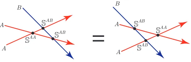
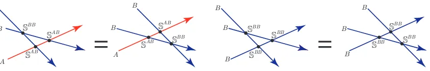
Consistency of the truncation means that the scattering of the lower-particle bound states (one- and two- in our present context) between themselves should fac-torise independently of the presence/absence of the higher-particle bound states. Thus, we require ˇS to satisfy the Yang-Baxter equation (3.39) which results in the following set of inequivalent equations for the individual S-matrices
SAA23 SAA13 SAA12 =SAA12 SAA13 SAA23 ,
SAB23 SAB13 SAA12 =SAA12 SAB13 SAB23 ,
SBB23 SAB13 SAB12 =SAB12 SAB13 SBB23 ,
SBB23 SBB13 SBB12 =SBB12 SBB13 SBB23 .
Here the first and the last equations are the standard Yang-Baxter equations for the S-matrices corresponding to scattering of the fundamental and the two-particle bound states respectively. The second and the third equations are defined in the spaces VA⊗VA⊗VB and V A⊗VB⊗VB correspondingly.
In the matrix language the properties of the S-matrix operator we discussed above take the following form.
Physical Unitarity.
S12g (z1∗, z2∗)†S12g (z1, z2) =I ⇐⇒ S12(z1∗, z2∗)†S12(z1, z2) =I ,
where S12g and S12 are defined in (3.20) and (3.21). CPT invariance.
S12g (z1, z2)T =S12g (z1, z2) ⇐⇒ S12(z1, z2)T =I12g S12(z1, z2)I12g ,
where the superscript “T” denotes the usual matrix transposition. Thus, the CPT invariance just means that the graded S-matrix is symmetric.
Parity Transformation.
S12g (z1, z2)−1 =I12g S
g
12(−z1,−z2)I12g ⇐⇒ S12(z1, z2)−1 =S12(−z1,−z2),
where the parity transformation acts on the S-matrix and any invariant operator as (S12g )P = I12g S12g I12g . This also means that in matrix language the grading of the tensor product of matrix unitiesEki⊗ELJ is defined to be (−1)ǫkǫL+ǫiǫJ.
Unitarity and Hermitian Analyticity.
In the general caseM 6=N
where
S21g,N M(z2, z1) =P12gS
g,N M
12 (z2, z1)P12g =
X
IKjl
SN M KlIj(z2, z1) (−1)ǫKǫl+ǫIǫjElj⊗EKI,
andP12g is the graded permutation matrix. The hermitian analyticity condition takes the form
S12g,M N(z1∗, z2∗)†=S21g,N M(z2, z1) ⇐⇒ S12M N(z1∗, z2∗)†=S21N M(z2, z1).
In the case M =N, we get SM M(z1, z2)→S12(z1, z2), and the unitarity and
hermi-tian analyticity conditions take the following form
S21g (z2, z1)S12g (z1, z2) =I ⇐⇒ S21(z2, z1)S12(z1, z2) =I ,
S12g (z1∗, z2∗)†=S21g (z2, z1) ⇐⇒ S12(z∗1, z2∗)† =S21(z2, z1),
where
S21g (z2, z1) =P12gS
g
12(z2, z1)P12g =
X
ikjl
Sijkl(z2, z1)(−1)ǫkǫl+ǫiǫjElj ⊗Eki,
and this means that the action of the graded permutation operator P is just given by the conjugation by the graded permutation matrix.
Yang-Baxter Equation. The operator YB equation (3.39) has the same matrix form only for the S-matrix S12 defined by (3.21):
S23S13S12 =S12S13S23,
where to simplify the notation we omit the explicit dependence of the S-matrices on
zi and Mi. To show this, we notice that the matrix form of the operators S12,S13
and S23 is
S12matr=S12g , S13matr =I23g S13g I23g , S23matr =I12g I13g S23g I13g I12g ,
where Sijg denotes the usual embedding of the matrix Sg into the product of three spaces. We see that the graded form of the S-matrix satisfies the following graded YB equation
I12g I13g S23g I13g I12g I23g S13g I23g S12g =S12g I23g S13g I23g I12g I13g S23g I13g I12g .
In terms of the S-matrix S12=I12g S12G the previous equation takes the form
I12g I13g I23g S23I12g I
g
23S13I23g I
g
12S12 =I12g S12I23g I
g
13S13I12g I
g
13S23I13g I
g
12.
Taking into account the identities
I12g I23g S13=S13I12g I
g
23, I
g
12I
g
13S23=S23I13g I
g
12,
we conclude thatS12 satisfies the usual YB equation. This completes our discussion
4. S-matrices
In this section we discuss the explicit construction and properties of the three S-matrices describing the scattering of fundamental particles and two-particle bound states.
4.1 The S-matrix SAA
As the warm-up exercise, here we will explain how to obtain the known scattering matrixSAA for fundamental particles [8, 12] in the framework of our new superspace approach.
According to our general discussion in section 3, the scattering matrixSAA is an
su(2)⊕su(2) invariant differential operator which acts on the tensor product of two fundamental multiplets
SAA : VA⊗V A → VA⊗VA.
Recall that
VA⊗V A=W 2,
whereW2 is a long irreducible supermultiplet of dimension 16 [19]. Under the action
of su(2)⊕su(2) this supermultiplet branches as follows
W2 = V0×V0+V0×V0+V1×V0+ (4.1)
+V0×V1 +V1/2×V1/2+V1/2×V1/2.
The 16-dimensional basis of the tensor product space VA⊗VA
VA⊗VA= Spannw1
awb2, wa1θ2α, wa1θ2α, θ1αθ2β
o
, a= 1,2; α= 3,4
can be easily adopted to the decomposition (4.1):
w1
awb2 = 1 2(w
1
aw2b −w1bw2a) + 1 2(w
1
aw2b +wb1w2a) → (V0+V1)×V0
wa1θα2 → V1/2×V1/2
wa2θα1 → V1/2×V1/2 θα1θ2β = 1
2(θ
1
αθβ2 −θ1βθα2) + 1 2(θ
1
αθβ2 +θβ1θα2) → V0×(V0+V1)
(4.2)
The space D2 of the second order differential operators dual to W2 branches under su(2)⊕su(2) in the same way:
D2 =D0×D0+D0×D0+D1×D0+ (4.3)
A basis adopted to this decomposition is formed by the following differential operators
ǫcd ∂ ∂wc
1
∂ ∂wd
2 →
D0×D0, ǫαβ
∂ ∂θα
1
∂
∂θβ2 → D
0 ×D0 ∂ ∂w2 a ∂ ∂θ1 α →
D1/2×D1/2, ∂ ∂w1
a
∂ ∂θ2
α →
D1/2×D1/2 ∂ ∂wa 1 ∂ ∂wb 2 + ∂ ∂wb 1 ∂ ∂wa 2 →
D1×D0, ∂
∂θα
1
∂ ∂θ2β +
∂ ∂θβ1
∂ ∂θα
2 →
D0×D1
(4.4)
The S-matrix we are looking for is an element of the space W2 ⊗D
2 which is
invariant under the action ofsu(2)⊕su(2). We obviously have
W2⊗D2 = (V0×V0+V0×V0+V1×V0+V0×V1+V1/2×V1/2+V1/2×V1/2)
⊗ (D0×D0+D0×D0+D1×D0+D0×D1+D12 ×D1/2+D1/2×D1/2) The invariants of su(2)⊕ su(2) arising in this tensor product decomposition are easy to count. Indeed, since Vj⊗Dj contains the singlet component (invariant), the
su(2)⊕su(2) invariants simply correspond to the singlet components of the spaces
Vj ⊗Dj ×Vk ⊗Dk in the tensor product decomposition of W 2 ⊗D
2. Thus, the
invariant subspace is generated by
Inv(W2⊗D2) = 4(V0⊗D0)×(V0⊗D0) + 4(V1/2⊗D1/2)×(V1/2⊗D1/2) +
+(V1⊗D1)×(V0⊗D0) + (V0⊗D0)×(V1⊗D1),
where integers in front of the spaces in the r.h.s of the last formulas indicate the corresponding multiplicities. Therefore, in the present case we find 10 invariant elements Λk in the space W2⊗D2. Their explicit form can be easily found by using
the bases (4.2) and (4.4):
Λ1=
1 2(w
1
awb2+w1bw2a)
∂2
∂w1
a∂wb2
, Λ7 =ǫabwa1wb2ǫαβ
∂2
∂θ2
β∂θ1α Λ2 =
1 2(w
1
awb2−wb1wa2)
∂2
∂w1
a∂wb2
, Λ8 =ǫαβθ1αθ2βǫab
∂2
∂w1
a∂wb2 Λ3 =
1 2(θ
1
αθβ2 +θ1βθ2α)
∂2
∂θ2
β∂θα1
, Λ9 =wa1θ2α
∂2
∂w2
a∂θα1 Λ4 =
1 2(θ
1
αθβ2 −θβ1θ2α)
∂2
∂θ2
β∂θ1α
, Λ10=w2aθα1
∂2
∂w1
a∂θ2α Λ5 =w1aθα2
∂2
∂w1
a∂θ2α
,
Λ6=w2aθα1
∂2
∂w2
a∂θ1α
.