The Second Dialog State Tracking Challenge
Matthew Henderson1, Blaise Thomson1 and Jason Williams2 1Department of Engineering, University of Cambridge, U.K.
2Microsoft Research, Redmond, WA, USA
[email protected] [email protected] [email protected]
Abstract
A spoken dialog system, while commu-nicating with a user, must keep track of what the user wants from the system at
each step. This process, termed dialog
state tracking, is essential for a success-ful dialog system as it directly informs the system’s actions. The first Dialog State Tracking Challenge allowed for evalua-tion of different dialog state tracking tech-niques, providing common testbeds and evaluation suites. This paper presents a second challenge, which continues this tradition and introduces some additional features – a new domain, changing user goals and a richer dialog state. The chal-lenge received 31 entries from 9 research groups. The results suggest that while large improvements on a competitive base-line are possible, trackers are still prone to degradation in mismatched conditions. An investigation into ensemble learning demonstrates the most accurate tracking can be achieved by combining multiple trackers.
1 Introduction
Spoken language provides a medium of communi-cation that is natural to users as well as hands- and eyes-free. Voice-based computer systems, called spoken dialog systems, allow users to interact us-ing speech to achieve a goal. Efficient operation of a spoken dialog system requires a component that can track what has happened in a dialog, incor-porating system outputs, user speech and context from previous turns. The building and evaluation of these trackers is an important field of research since the performance of dialog state tracking is important for the final performance of a complete system.
Until recently, it was difficult to compare ap-proaches to state tracking because of the wide va-riety of metrics and corpora used for evaluation. The first dialog state tracking challenge (DSTC1) attempted to overcome this by defining a challenge task with standard test conditions, freely available corpora and open access (Williams et al., 2013). This paper presents the results of a second chal-lenge, which continues in this tradition with the inclusion of additional features relevant to the re-search community.
Some key differences to the first challenge in-clude:
• The domain is restaurant search instead of
bus timetable information. This provides par-ticipants with a different category of interac-tion where there is a database of matching en-tities.
• Users’ goals are permitted to change. In the
first challenge, the user was assumed to al-ways want a specific bus journey. In this chal-lenge the user’s goal can change. For exam-ple, they may want a ‘Chinese’ restaurant at the start of the dialog but change to wanting ‘Italian’ food by the end.
• The dialog state uses a richer
representa-tion than in DSTC1, including not only the slot/value attributes of the user goal, but also their search method, and what information they wanted the system to read out.
As well as presenting the results of the different state trackers, this paper attempts to obtain some insights into research progress by analysing their performance. This includes analyses of the predic-tive power of performance on the development set, the effects of tracking the dialog state using joint distributions, and the correlation between 1-best accuracy and overall quality of probability distri-butions output by trackers. An evaluation of the effects of ensemble learning is also performed.
The paper begins with an overview of the
lenge in section 2. The labelling scheme and met-rics used for evaluation are discussed in section 3 followed by a summary of the results of the chal-lenge in section 4. An analysis of ensemble learn-ing is presented in section 5. Section 6 concludes the paper.
2 Challenge overview
2.1 Problem statement
This section defines the problem of dialog state tracking as it is presented in the challenge. The challenge evaluates state tracking for dialogs where users search for restaurants by specifying constraints, and may ask for information such as the phone number. The dialog state is formu-lated in a manner which is general to information browsing tasks such as this.
Included with the data is an ontology1, which
gives details of all possible dialog states. The
ontology includes a list of attributes termed
re-questable slotswhich the user may request, such
as the food type or phone number. It also provides
a list ofinformable slotswhich are attributes that
may be provided as constraints. Each informable slot has a set of possible values. Table 1 gives de-tails on the ontology used in DSTC2.
The dialog state at each turn consists of three components:
• Thegoal constraintfor eachinformableslot.
This is either an assignment of a value from the ontology which the user has specified as a constraint, or is a special value — either
Dontcarewhich means the user has no
pref-erence, orNonewhich means the user is yet
to specify a valid goal for this slot.
• A set of requested slots, i.e. those slots
whose values have been requested by the user, and should be informed by the system.
• An assignment of the current dialogsearch
method. This is one of
– by constraints, if the user is attempting
to issue a constraint,
– by alternatives, if the user is requesting
alternative suitable venues,
– by name, if the user is attempting to ask
about a specific venue by its name,
– finished, if the user wants to end the call
– ornoneotherwise.
Note that in DSTC1, the set of dialog states 1Note that this ontology includes only the schema for
di-alog states and not the database entries
was dependent on the hypotheses given by a Spo-ken Language Understanding component (SLU) (Williams et al., 2013), whereas here the state is labelled independently of any SLU (see section 3). Appendix B gives an example dialog with the state labelled at each turn.
A tracker must use information up to a given turn in the dialog, and output a probability distri-bution over dialog states for the turn. Trackers output separately the distributions for goal con-straints, requested slots and the method. They may either report a joint distribution over the goal con-straints, or supply marginal distributions and let the joint goal constraint distribution be calculated as a product of the marginals.
2.2 Challenge design
DSTC2 studies the problem of dialog state track-ing as a corpus-based task, similar to DSTC1. The challenge task is to re-run dialog state tracking over a test corpus of dialogs.
A corpus-based challenge means all trackers are evaluated on the same dialogs, allowing di-rect comparison between trackers. There is also no need for teams to expend time and money in building an end-to-end system and getting users, meaning a low barrier to entry.
When a tracker is deployed, it will inevitably al-ter the performance of the dialog system it is part of, relative to any previously collected dialogs. In order to simulate this, and to penalise overfitting to known conditions, evaluation dialogs in the chal-lenge are drawn from dialogs with a dialog man-ager which is not found in the training data. 2.3 Data
A large corpus of dialogs with various telephone-based dialog systems was collected using Ama-zon Mechanical Turk. The dialogs used in the challenge come from 6 conditions; all combina-tions of 3 dialog managers and 2 speech recognis-ers. There are roughly 500 dialogs in each condi-tion, of average length 7.88 turns from 184 unique callers.
The 3 dialog managers are:
• DM-HC, a simple tracker maintaining a
sin-gle top dialog state, and a hand-crafted policy
• DM-POMDPHC, a dynamic Bayesian
net-work for tracking a distribution of dialog states, and a hand-crafted policy
• DM-POMDP, the same tracking method as
Slot Requestable Informable
area yes yes. 5 values; north,south, east, west, centre food yes yes, 91 possible values name yes yes, 113 possible values pricerange yes yes, 3 possible values
addr yes no
phone yes no
postcode yes no
[image:3.595.76.284.62.168.2]signature yes no
Table 1: Ontology used in DSTC2 for restaurant
informa-tion. Counts do not include the specialDontcarevalue.
POMDP reinforcement learning The 2 speech recognisers are:
• ASR-degraded, speech recogniser with
arti-ficially degraded statistical acoustic models
• ASR-good, full speech recogniser optimised
for the domain
These give two acoustic conditions, the de-graded model producing dialogs at higher error rates. The degraded models simulate in-car con-ditions and are described in Young et al. (2013).
The set of all calls with DM-POMDP, with both speech recognition configurations, constitutes the test set. All calls with the other two dialog man-agers are used for the training and development set. Specifically, the datasets are arranged as so:
• dstc2 train. Labelled dataset released in
Oc-tober 2013, with 1612 calls from DM-HC and DM-POMDPHC, and both ASR conditions.
• dstc2 dev. Labelled dataset released at the
same time as dstc2 train, with 506 calls under the same conditions as dstc2 train. No caller in this set appears in dstc2 train.
• dstc2 test. Set used for evaluation. Released
unlabelled at the beginning of the evaluation week. This consists of all 1117 dialogs with DM-POMDP.
Paid Amazon Mechanical Turkers were as-signed tasks and asked to call the dialog systems. Callers were asked to find restaurants that matched particular constraints on the slots area, pricerange and food. To elicit more complex dialogs, includ-ing changinclud-ing goals (goals in DSTC1 were always constant), the users were sometimes asked to find more than one restaurant. In cases where a match-ing restaurant did not exist they were required to seek an alternative, for example finding an Indian instead of an Italian restaurant.
A breakdown of the frequency of goal con-straint changes is given in table 2, showing around 40% of all dialogs involved a change in goal con-straint. The distribution of the goal constraints in
50 100 150 200
Figure 1: Histogram of values for the food constraint
(ex-cluding dontcare) in all data. The most frequent values are Indian, Chinese, Italian and European.
Dataset
train dev test
area 2.9% 1.4% 3.8%
food 37.3% 34.0% 40.9%
name 0.0% 0.0% 0.0%
pricerange 1.7% 1.6% 3.1%
any 40.1% 37.0% 44.5%
Table 2: Percentage of dialogs which included a change in
the goal constraint for each informable (and any slot). Barely any users asked for restaurants by name.
the data was reasonably uniform across the area and pricerange slots, but was skewed for food as shown in figure 1. The skew arises from the distri-bution of the restaurants in the system’s database; many food types have very few matching venues.
Recently, researchers have started using word confusion networks for spoken language under-standing (Henderson et al., 2012; T¨ur et al., 2013). Unfortunately, word confusion networks were not logged at the time of collecting the dialog data. In order to provide word confusion networks, ASR was run offline in batch mode on each dialog us-ing similar models as the live system. This gives
a second set of ASR results, labelledbatch, which
not only includes ASRN-best lists (as inlive
re-sults), but also word confusion networks.
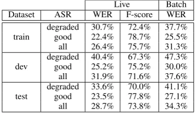
For each dataset and speech recogniser, table 3 gives the Word Error Rate on the top ASR hypoth-esis, and F-score for the top SLU hypothesis (cal-culated as in Henderson et al. (2012)). Note the batch ASR was always less accurate than the live.
Live Batch
Dataset ASR WER F-score WER
train degradedgood 30.7%22.4% 72.4%78.7% 37.7%25.5%
all 26.4% 75.7% 31.3%
dev degradedgood 40.4%25.2% 67.3%75.2% 47.3%30.0%
all 31.9% 71.6% 37.6%
test degradedgood 33.6%23.5% 70.0%77.8% 41.1%27.1%
[image:3.595.336.496.176.250.2]all 28.7% 73.8% 34.3%
Table 3:Word Error Rate on the top hypothesis, and F-score
[image:3.595.317.516.622.737.2]3 Labelling and evaluation
The output of each tracker is a distribution over dialog states for each turn, as explained in section 2.1. To allow evaluation of the tracker output, the single correct dialog state at each turn is labelled.
Labelling of the dialog state is facilitated by first labelling each user utterance with its semantic rep-resentation, in the dialog act format described in Henderson et al. (2013) (some example seman-tic representations are given in appendix B). The semantic labelling was achieved by first crowd-sourcing the transcription of the audio to text. Next a semantic decoder was run over the tran-scriptions, and the authors corrected the decoder’s results by hand. Given the sequence of machine actions and user actions, both represented seman-tically, the true dialog state is computed determin-istically using a simple set of rules.
Recall the dialog state is composed of multiple components; the goal constraint for each slot, the requested slots, and the method. Each of these is evaluated separately, by comparing the tracker output to the correct label. The joint over the goal constraints is evaluated in the same way, where the tracker may either explicitly enumerate and score its joint hypotheses, or let the joint be computed as the product of the distributions over the slots.
A bank of metrics which look at the tracker out-put and the correct labels are calculated in the eval-uation. These metrics are a slightly expanded set of those calculated in DSTC1.
Denote an example probability distribution
given by a tracker aspand the correct label to be
i, so we have that the probability reported to the
correct hypothesis ispi, andPjpj = 1.
Accuracymeasures the fraction of turns where
the top hypothesis is correct, i.e. where i =
arg maxjpj. AvgP, average probability,
mea-sures the mean score of the correct hypothesis,pi.
This gives some idea of the quality of the score given to the correct hypothesis, ignoring the rest
of the distribution. Neglogp is the mean
nega-tive logarithm of the score given to the correct
hy-pothesis,−logpi. Sometimes called thenegative
log likelihood, this is a standard score in machine
learning tasks. MRRis the mean reciprocal rank
of the top hypothesis, i.e. 1+1k wherejk = iand
pj0 ≥ pj1 ≥. . .. This metric measures the
qual-ity of the ranking, without necessarily treating the
scores as probabilities. L2 measures the square
of the l2 norm between the distribution and the
correct label, indicating quality of the whole re-ported distribution. It is calculated for one turn
as (1−pi)2 +Pj6=ip2j. Two metrics, Update
precision andUpdate accuracymeasure the
ac-curacy and precision of updates to the top scoring hypothesis from one turn to the next. For more details, see Higashinaka et al. (2004), which finds these metrics to be highly correlated with dialog success in their data.
Finally there is a set of measures relating to the receiver operating characteristic (ROC) curves, which measure the discrimination of the scores for the highest-ranked hypotheses. Two versions of ROC are computed, V1 and V2. V1 computes correct-accepts (CA), false accepts (FA) and
false-rejects (FR) as fractions of all utterances. The
V2 metrics consider fractions of correctly classi-fied utterances, meaning the values always reach 100% regardless of the accuracy. V2 metrics mea-sure discrimination independently of the accuracy, and are therefore only comparable between track-ers with similar accuracies.
Several metrics are computed from the ROC
statistics. ROC V1 EER computes the false
ac-ceptance rate at the point where false-accepts are
equal to false-rejects. ROC V1 CA05,ROC V1
CA10,ROC V1 CA20andROC V2 CA05,ROC
V2 CA10, ROC V2 CA20, compute the correct
acceptance rates for both versions of ROC at false-acceptance rates 0.05, 0.10, and 0.20.
Twoschedulesare used to decide which turns to
include when computing each metric.Schedule 1
includes every turn. Schedule 2 only includes a
turn if any SLU hypothesis up to and including the turn contains some information about the compo-nent of the dialog state in question, or if the correct
label is notNone. E.g. for a goal constraint, this is
whether the slot has appeared with a value in any SLU hypothesis, an affirm/negate act has appeared after a system confirmation of the slot, or the user has in fact informed the slot regardless of the SLU. The data is labelled using two schemes. The
first, scheme A, is considered the standard
la-belling of the dialog state. Under this scheme, each component of the state is defined as the most recently asserted value given by the user. The
Nonevalue is used to indicate that a value is yet
to be given. Appendix B demonstrates labelling under scheme A.
A second labelling scheme, scheme B, is
prop-agated backwards through the dialog. This la-belling scheme is designed to assess whether a tracker is able to predict a user’s intention be-fore it has been stated. Under scheme B, the la-bel at a current turn for a particular component of the dialog state is considered to be the next value which the user settles on, and is reset in the case of goal constraints if the slot value pair is given in
acanthelp act by the system (i.e. the system has
informed that this constraint is not satisfiable).
3.1 Featured metrics
All combinations of metrics, state components, schedules and labelling schemes give rise to 815 total metrics calculated per tracker in evaluation. Although each may have its particular motiva-tion, many of the metrics will be highly corre-lated. From the results of DSTC1 it was found the metrics could be roughly split into 3 indepen-dent groups; one measuring 1-best quality (e.g. Acc), another measuring probability calibration (e.g. L2), and the last measuring discrimination (e.g. ROC metrics) (Williams et al., 2013).
By selecting a representative from each of these groups, the following were chosen as featured metrics:
• Accuracy, schedule 2, scheme A
• L2 norm, schedule 2, scheme A
• ROC V2 CA 5, schedule 2, scheme A
Accuracy is a particularly important measure for dialog management techniques which only consider the top dialog state hypothesis at each turn, while L2 is of more importance when mul-tiple dialog states are considered in action selec-tion. Note that the ROC metric is only compara-ble among systems operating at similar accuracies, and while L2 should be minimised, Accuracy and the ROC metric should be maximised.
Each of these, calculated for joint goal
con-straints, search method and combined
re-quested slots, gives 9 metrics altogether which
participants were advised to focus on optimizing.
3.2 Baseline trackers
Three baseline trackers were entered in the chal-lenge, under the ID ‘team0’. Source code for all the baseline systems is available on the DSTC
website2. The first, ‘team0.entry0’, follows
sim-ple rules commonly used in spoken dialog sys-tems. It gives a single hypothesis for each slot,
2http://camdial.org/˜mh521/dstc/
whose value is the top scoring suggestion so far in the dialog. Note that this tracker does not account well for goal constraint changes; the hypothesised value for a slot will only change if a new value occurs with a higher confidence.
The focusbaseline, ‘team0.entry1’, includes a
simple model of changing goal constraints.
Be-liefs are updated for the goal constraints= v, at
turnt,P(s=v), using the rule:
P(s=v)t=qtP(s=v)t−1+SLU(s=v)t
where 0 ≤ SLU(s = v)t ≤ 1 is the evidence
for s = v given by the SLU in turnt, and qt =
P
v0SLU(s=v0)t≤1.
Another baseline tracker, based on the tracker presented in Wang and Lemon (2013) is included in the evaluation, labelled ‘team0.entry2’. This tracker uses a selection of domain independent rules to update the beliefs, similar to the focus baseline. One rule uses a learnt parameter called the noise adjustment, to adjust the SLU scores. Full details of this and all baseline trackers are pro-vided on the DSTC website.
Finally, an oracle tracker is included under the label ‘team0.entry3’. This reports the correct la-bel with score 1 for each component of the dialog state, but only if it has been suggested in the dialog so far by the SLU. This gives an upper-bound for the performance of a tracker which uses only the SLU and its suggested hypotheses.
4 Results
Altogether 9 research teams participated in the challenge. Each team could submit a maximum of 5 trackers, and 31 trackers were submitted in total. Teams are identified by anonymous team numbers team1-9, and baseline systems are grouped under team0. Appendix A gives the results on the fea-tured metrics for each entry submitted to the chal-lenge. The full results, including tracker output, details of each tracker and scripts to run the evalu-ation are available on the DSTC2 website.
The table in appendix A specifies which of the inputs available were used for each tracker- from live ASR, live SLU and batch ASR. This facil-itates comparisons between systems which used the same information.
For the “requested slot” task, some trackers out-performed the oracle tracker. This was possible because trackers could guess a slot was requested using dialog context, even if there was no mention of it in the SLU output.
[image:6.595.309.492.209.432.2]Participants were asked to report the results of their trackers on the dstcs2 dev development set. Figure 2 gives some insight into how well mance on the development set predicted perfor-mance on the test set. Metrics are reported as per-centage improvement relative to the focus base-line to normalise for the difficulty of the datasets; in general trackers achieved higher accuracies on the test set than on development. Figure 2 shows that the development set provided reasonable pre-dictions, though in all cases improvement rel-ative to the baseline was overestimated, some-times drastically. This suggests that approaches to tracking have trouble with generalisation, under-performing in the mismatched conditions of the test set which used an unseen dialog manager.
Joint Goal Constraint Accuracy
0.3 0.2 0.1 0.1
team1entry0 team2entry1 team3entry0 team4entry0 team5entry4 team6entry2 team7entry0 team8entry1 team9entry0
Joint Goal Constraint L2
team1entry0 team2entry1 team3entry0 team4entry0 team5entry4 team6entry2 team7entry0 team8entry1 team9entry0
[image:6.595.75.239.360.573.2]0.2 0.2 0.4 0.6
Figure 2: Performance relative to the focus baseline
(per-centage increase) for dev set (white) and test set (grey). Top entry for each team chosen based on joint goal constraint ac-curacy. A lower L2 score is better.
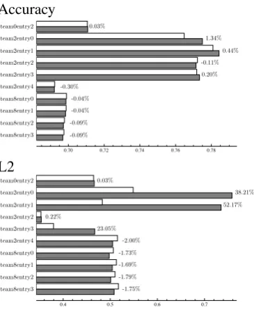
Recall from section 2, trackers could output joint distributions for goal constraints, or simply output one distribution for each slot and allow the joint to be calculated as the product. Two teams, team2 and team8, opted to output a joint distribu-tion for some of their entries. Figure 3 compares performance on the test set for these trackers be-tween the joint distributions they reported, and the joint calculated as the product. The entries from team2 were able to show an increase in the
accu-racy of the top joint goal constraint hypotheses, but seemingly at a cost in terms of the L2 score. Conversely the entries from team8, though oper-ating at lower performance than the focus base-line, were able to show an improvement in L2 at a slight loss in accuracy. These results suggest that a tracking method is yet to be proposed which can, at least on this data, improve both accuracy and the L2 score of tracker output by reporting joint predictions of goal constraints.
Accuracy team0entry2 team2entry0 team2entry1 team2entry2 team2entry3 team2entry4 team8entry0 team8entry1 team8entry2 team8entry3
0.70 0.72 0.74 0.76 0.78
0.03% 1.34% 0.44% -0.11% 0.20% -0.30% -0.04% -0.09% -0.04% -0.09% L2 team0entry2 team2entry0 team2entry1 team2entry3 team2entry4 team8entry0 team8entry1 team8entry2 team8entry3 team8entry4
0.4 0.5 0.6 0.7
team0entry2 team2entry0 team2entry1 team2entry2 team2entry3 team2entry4 team8entry0 team8entry1 team8entry2 team8entry3 0.03% 38.21% 52.17% 0.22% 23.05% -2.00% -1.73% -1.69% -1.79% -1.75%
Figure 3: Influence of reporting a full joint distribution.
White bar shows test set performance computing the goal constraints as a product of independent marginals; dark bar is performance with a full joint distribution. All entries which reported a full joint are shown. A lower L2 score is better.
It is of interest to investigate the correlation be-tween accuracy and L2. Figure 4 plots these met-rics for each tracker on joint goal constraints. We see that in general a lower L2 score correlates with a higher accuracy, but there are examples of high accuracy trackers which do poorly in terms of L2. This further justifies the reporting of these as two separate featured metrics.
0.50 0.55 0.60 0.65 0.70 0.75 0.80 0.3 0.4 0.5 0.6 0.7 0.8 team2entry0 team2entry1 team4entry0 team2entry3 focus baseline, team0entry2
Accuracy
[image:6.595.326.504.622.734.2]L2
Figure 4: Scatterplot of joint goal constraint accuracy and
Joint goal Method Requested
Tracker Acc. L2 Acc. L2 Acc. L2
[image:7.595.125.468.62.176.2]Single best entry 0.784 0.346 0.950 0.082 0.978 0.035 Score averaging: top 2 entries 0.787 0.364- 0.945- 0.083 0.976 0.039-Score averaging: top 5 entries 0.777 0.347 0.945 0.089- 0.976 0.038 Score averaging: top 10 entries 0.760- 0.364- 0.934- 0.108- 0.967- 0.056-Score averaging: all entries 0.765- 0.362- 0.934- 0.103- 0.971- 0.052-Stacking: top 2 entries 0.789 0.322+ 0.949 0.085- 0.977 0.040-Stacking: top 5 entries 0.795+ 0.315+ 0.949 0.084 0.978 0.037 Stacking: top 10 entries 0.796+ 0.312+ 0.949 0.083 0.979 0.035 Stacking: all entries 0.798+ 0.308+ 0.950 0.083 0.980 0.034
Table 4: Accuracy and L2 for Joint goal constraint, Method, and Requested slots for the single best tracker (by accuracy) in
DSTC2, and various ensemble methods. “Top N entries” means the N entries with highest accuracies from distinct teams, where the baselines are included as a team. +/- indicates statistically significantly better/worse than the single best entry (p <0.01), computed with McNemar’s test for accuracy and the paired t-test for L2, both with Bonferroni correction for repeated tests.
5 Ensemble learning
The dialog state tracking challenge provides an
opportunity to studyensemble learning– i.e.
syn-thesizing the output of many trackers to improve performance beyond any single tracker. Here we
consider two forms of ensemble learning: score
averagingandstacking.
In score averaging, the final score of a class is computed as the mean of the scores output by all trackers for that class. One of score averaging’s strengths is that it requires no additional training data beyond that used to train the constituent track-ers. If each tracker’s output is correct more than half the time, and if the errors made by trackers are not correlated, then score averaging is guaranteed to improve performance (since the majority vote will be correct in the limit). In (Lee and Eskenazi, 2013), score averaging (there called “system com-bination”) has been applied to combine the output of four dialog state trackers. To help decorrelate errors, constituent trackers were trained on differ-ent subsets of data, and used differdiffer-ent machine learning methods. The relative error rate reduction
was5.1%on the test set.
The second approach to ensemble learning is stacking (Wolpert, 1992). In stacking, the scores output by the constituent classifiers are fed to a
new classifier that makes a final prediction. In
other words, the output of each constituent
classi-fier is viewed as afeature, and the new final
classi-fier can learn the correlations and error patterns of each. For this reason, stacking often outperforms score averaging, particularly when errors are cor-related. However, stacking requires a validation set for training the final classifier. In DSTC2, we only have access to trackers’ output on the test set. Therefore, to estimate the performance of stack-ing, we perform cross-validation on the test set: the test set is divided into two folds. First, fold 1
is used for training the final classifier, and fold 2 is used for testing. Then the process is reversed. The two test outputs are then concatenated. Note that models are never trained and tested on the same data. A maximum entropy model (maxent) is used (details in (Metallinou et al., 2013)), which is common practice for stacking classifiers. In addi-tion, maxent was found to yield best performance in DSTC1 (Lee and Eskenazi, 2013).
Table 4 reports accuracy and L2 for goal con-straints, search method, and requested slots. For each ensemble method and each quantity (column) the table gives results for combining the top track-ers from 2 or 5 distinct teams, for combining the top tracker from each team, and combining all trackers (including the baselines as a team). For example, the joint goal constraint ensemble with the top 2 entries was built from team2.entry1 & team4.entry0, and the method ensemble with the top 2 entries from team2.entry4 & team4.entry0.
Table 4 shows two interesting trends. The first is that score averaging does not improve perfor-mance, and performance declines as more track-ers are combined, yielding a statistically signifi-cant decrease across all metrics. This suggests that the errors of the different trackers are correlated, which is unsurprising since they were trained on the same data. On the other hand, stacking yields a statistically significant improvement in accuracy for goal constraints, and doesn’t degrade accuracy for the search method and requested slots. For stacking, the trend is that adding more trackers in-creases performance – for example, combining the best tracker from every team improves goal con-straint accuracy from 78.4% to 79.8%.
mag-nitude of that improvement, so it is an open
ques-tion whether stacking is thebestuse of additional
data. Also, the training and test conditions of the final stacking classifier are not mis-matched, whereas in practice they would be. Nonethe-less, this result does suggest that, if additional data is available, stacking can be used to success-fully combine multiple trackers and achieve per-formance better than the single best tracker.
6 Conclusions
DSTC2 continues the tradition of DSTC1 by pro-viding a common testbed for dialog state track-ing, introducing some additional features relevant to the research community– specifically a new domain, changing user goals and a richer dialog state. The data, evaluation scripts, and baseline trackers will remain available and open to the re-search community online.
Results from the previous challenge motivated
the selection of a few metrics as featured
met-rics, which facilitate comparisons between track-ers. Analysis of the performance on the matched development set and the mismatched test set sug-gests that there still appears to be limitations on generalisation, as found in DSTC1. The results also suggest there are limitations in exploiting cor-relations between slots, with few teams exploiting joint distributions and the effects of doing so being mixed. Investigating ensemble learning demon-strates the effectiveness of combining tracker out-puts. Ensemble learning exploits the strengths of individual trackers to provide better quality output than any constituent tracker in the group.
A follow up challenge, DSTC3, will present the problem of adapting to a new domain with very few example dialogs. Future work should also verify that improvements in dialog state track-ing translate to improvements in end-to-end dia-log system performance. In this challenge, paid subjects were used as users with real information needs were not available. However, differences between these two user groups have been shown (Raux et al., 2005), so future studies should also test on real users.
Acknowledgements
The authors thank the advisory committee for their valuable input: Paul Crook, Maxine Eske-nazi, Milica Gaˇsi´c, Helen Hastie, Kee-Eung Kim, Sungjin Lee, Oliver Lemon, Olivier Pietquin, Joelle Pineau, Deepak Ramachandran, Brian
Strope and Steve Young. The authors also thank Zhuoran Wang for providing a baseline tracker, and DJ Kim, Sungjin Lee & David Traum for com-ments on evaluation metrics. Finally, thanks to SIGdial for their endorsement, and to the partic-ipants for making the challenge a success.
References
Matthew Henderson, Milica Gaˇsi´c, Blaise Thom-son, Pirros Tsiakoulis, Kai Yu, and Steve Young. 2012. Discriminative Spoken Language
Under-standing Using Word Confusion Networks. In
Spo-ken Language Technology Workshop, 2012. IEEE.
Matthew Henderson, Blaise Thomson, and Jason Williams. 2013. Dialog State Tracking Challenge 2 & 3 Handbook. camdial.org/˜mh521/dstc/. Ryuichiro Higashinaka, Noboru Miyazaki, Mikio
Nakano, and Kiyoaki Aikawa. 2004. Evaluat-ing discourse understandEvaluat-ing in spoken dialogue
sys-tems. ACM Trans. Speech Lang. Process.,
Novem-ber.
Sungjin Lee and Maxine Eskenazi. 2013. Recipe for building robust spoken dialog state trackers: Dialog
state tracking challenge system description. In
Pro-ceedings of the SIGDIAL 2013 Conference.
Angeliki Metallinou, Dan Bohus, and Jason D. Williams. 2013. Discriminative state tracking for
spoken dialog systems. In Proc Association for
Computational Linguistics, Sofia.
Antoine Raux, Brian Langner, Dan Bohus, Alan W Black, and Maxine Eskenazi. 2005. Let’s go public! Taking a spoken dialog system to the real world. G¨okhan T¨ur, Anoop Deoras, and Dilek Hakkani-T¨ur.
2013. Semantic parsing using word confusion
net-works with conditional random fields. In
INTER-SPEECH.
Zhuoran Wang and Oliver Lemon. 2013. A simple and generic belief tracking mechanism for the dia-log state tracking challenge: On the believability of
observed information. In Proceedings of the
SIG-DIAL 2013 Conference.
Jason Williams, Antoine Raux, Deepak Ramachadran, and Alan Black. 2013. The Dialog State
Track-ing Challenge. InProceedings of the SIGDIAL 2013
Conference, Metz, France, August.
David H. Wolpert. 1992. Stacked generalization.
Neu-ral Networks, 5:241–259.
Steve Young, Catherine Breslin, Milica Gaˇsi´c, Matthew Henderson, Dongho Kim, Martin Szum-mer, Blaise Thomson, Pirros Tsiakoulis, and Eli Tzirkel Hancock. 2013. Evaluation of Statistical POMDP-based Dialogue Systems in Noisy
Environ-ment. InProceedings of IWSDS, Napa, USA,
Appendix A: Featured results of evaluation
Tracker Inputs Joint Goal Constraints Search Method Requested Slots
team entry LiveASR LiveSLU BatchASR Acc L2 ROC Acc L2 ROC Acc L2 ROC
0* 0 X 0.619 0.738 0.000 0.879 0.209 0.000 0.884 0.196 0.000
1 X 0.719 0.464 0.000 0.867 0.210 0.349 0.879 0.206 0.000
2 X 0.711 0.466 0.000 0.897 0.158 0.000 0.884 0.201 0.000
3 X† 0.850 0.300 0.000 0.986 0.028 0.000 0.957 0.086 0.000
1 0 X 0.601 0.649 0.064 0.904 0.155 0.187 0.960 0.073 0.000
1 X 0.596 0.671 0.036 0.877 0.204 0.397 0.957 0.081 0.000
2 0 X X 0.775 0.758 0.063 0.944 0.092 0.306 0.954 0.073 0.383
1 X X X 0.784 0.735 0.065 0.947 0.087 0.355 0.957 0.068 0.446
2 X 0.668 0.505 0.249 0.944 0.095 0.499 0.972 0.043 0.300
3 X X X 0.771 0.354 0.313 0.947 0.093 0.294 0.941 0.090 0.262
4 X X X 0.773 0.467 0.140 0.950 0.082 0.351 0.968 0.050 0.497
3 0 X 0.729 0.452 0.000 0.878 0.210 0.000 0.889 0.188 0.000
4 0 X 0.768 0.346 0.365 0.940 0.095 0.452 0.978 0.035 0.525
1 X 0.746 0.381 0.383 0.939 0.097 0.423 0.977 0.038 0.490
2 X 0.742 0.387 0.345 0.922 0.124 0.447 0.957 0.069 0.340
3 X 0.737 0.406 0.321 0.922 0.125 0.406 0.957 0.073 0.385
5 0 X X 0.686 0.628 0.000 0.889 0.221 0.000 0.868 0.264 0.000
1 X X 0.609 0.782 0.000 0.927 0.147 0.000 0.974 0.053 0.000
2 X X 0.637 0.726 0.000 0.927 0.147 0.000 0.974 0.053 0.000
3 X X 0.609 0.782 0.000 0.927 0.147 0.000 0.974 0.053 0.000
4 X X 0.695 0.610 0.000 0.927 0.147 0.000 0.974 0.053 0.000
6 0 X 0.713 0.461 0.100 0.865 0.228 0.199 0.932 0.118 0.057
1 X 0.707 0.447 0.223 0.871 0.211 0.290 0.947 0.093 0.218
2 X 0.718 0.437 0.207 0.871 0.210 0.287 0.951 0.085 0.225
7 0 X 0.750 0.416 0.081 0.936 0.105 0.237 0.970 0.056 0.000
1 X 0.739 0.428 0.159 0.921 0.161 0.554 0.970 0.056 0.000
2 X 0.750 0.416 0.081 0.929 0.117 0.379 0.971 0.054 0.000
3 X 0.725 0.432 0.105 0.936 0.105 0.237 0.972 0.047 0.000
4 X 0.735 0.433 0.086 0.910 0.140 0.280 0.946 0.089 0.190
8 0 X 0.692 0.505 0.071 0.899 0.153 0.000 0.935 0.106 0.000
1 X 0.699 0.498 0.067 0.899 0.153 0.000 0.939 0.101 0.000
2 X 0.698 0.504 0.067 0.899 0.153 0.000 0.939 0.101 0.000
3 X 0.697 0.501 0.068 0.899 0.153 0.000 0.939 0.101 0.000
4 X 0.697 0.508 0.068 0.899 0.153 0.000 0.939 0.101 0.000
9 0 X 0.499 0.760 0.000 0.857 0.229 0.000 0.905 0.149 0.000
* The entries under team0 are the baseline systems mentioned in section 3.2. † team0.entry3 is the
oracle tracker, which uses the labels on the test set and limits itself to hypotheses suggested by the live SLU.
Appendix B: Sample dialog, labels, and tracker output
S:
U:
Which part of town?
The north uh area
0.2 inform(food=north_african) area=north
method=byconstraints
requested=() 0.1 inform(area=north)
0.2 food=north_african
0.1 area=north
request(area)
inform(area=north) 0.9 byconstraints0.1 none
0.0 phone 0.0 address
Actual input and output SLU hypotheses and scores Labels Example tracker output Correct?
S:
U:
Which part of town?
A cheap place in the north
inform(area=north, pricerange=cheap)
0.8 inform(area=north), inform(pricerange=cheap)
area=north pricerange=cheap
method=byconstraints
requested=() 0.1 inform(area=north)
0.7 area=north pricerange=cheap 0.1 area=north
food=north_african
request(area)
0.9 byconstraints 0.1 none
0.0 phone 0.0 address
S:
U:
Clown café is a cheap restaurant in the north part of town. Do you have any others like that, maybe in the south part of town?
reqalts(area=south)
0.7 reqalts(area=south) area=south
pricerange=cheap
method=byalternatives
requested=() 0.2 reqmore()
0.8 area=south pricerange=cheap 0.1 area=north
pricerange=cheap
0.6 byalternatives 0.2 byconstraints
0.0 phone 0.0 address
S:
U:
Galleria is a cheap restaurant in the south.
What is their phone number and address?
request(phone), request(address)
0.6 request(phone) area=south
pricerange=cheap
method=byalternatives
requested= (phone, address) 0.2 request(phone),
request(address)
0.9 area=south pricerange=cheap 0.1 area=north
pricerange=cheap
0.5 byconstraints
0.4 byalternatives
0.8 phone 0.3 address 0.1 request(address)
0.7 ()
0.2 ()
0.1 ()
0.0 ()