Munich Personal RePEc Archive
A simple new test for slope homogeneity
in panel data models with interactive
effects
Ando, Tomohiro and Bai, Jushan
Keio University, Columbia University
21 December 2014
Online at
https://mpra.ub.uni-muenchen.de/60994/
A simple new test for slope homogeneity in panel
data models with interactive effects
December 20, 2014
Tomohiro Ando
Jushan Bai
Keio University
Columbia University
Abstract
We consider the problem of testing for slope homogeneity in high-dimensional panel data models with cross-sectionally correlated errors. We consider a Swamy-type test for slope homogeneity by incorporating interactive fixed effects. We show that the pro-posed test statistic is asymptotically normal. Our test allows the explanatory variables to be correlated with the unobserved factors, factor loadings, or with both. Monte Carlo simulations demonstrate that the proposed test has good size control and good power.
Key words: Cross-sectional dependence, Endogenous predictors, Slope homogeneity
1
Introduction
This paper considers the testing of slope homogeneity for high-dimensional panel data models. Testing slope homogeneity is useful for empirical studies. In finance, for example, testing asset pricing models, including the capital asset pricing model1
and the multiple factor pricing models,2 is related to testing homogeneity.3 There are a number
of studies on testing for slope homogeneity in panel data models, including Pesaran et al. (1996), Phillips and Sul (2003), Pesaran and Yamagata (2008), Blomquist and Westerlund (2013), and Su and Chen (2013).
Pesaran and Yamagata’s (2008) testing procedure is useful in the sense that it treats a high-dimensional panel data model where the number of cross-sectional unitsN and the time series dimensionT are large. However, the test does not allow cross-sectionally, serially correlated errors. To deal with the serially correlated errors, Blomquist and Westerlund (2013) extended their test to the case when the errors are heteroskedastic and/or serially correlated in an unknown fashion. However, the test still does not deal with the practically relevant case of cross-sectional dependence. Moreover, these tests do not allow dependence between the set of predictors and unobservable errors.
To deal with these problems, we propose a new simple test that accommodates cross-sectional dependence by using the results of Bai (2009), Song (2013), and Ando and Bai (2014). These studies considered panel data models with interactive fixed effects. Our proposed test statistic, denoted by ˆΓ, is a modified version of Swamy’s (1970) test statistic, similar to that of Pesaran and Yamagata (2008). An advantage of our testing procedure is that it provides a robust test under cross-sectionally correlated errors with heteroskedasticity. Furthermore, the proposed test works even when the set of predictors and the unobservable errors that contain the factor structure are correlated. We investigate the asymptotic distribution of our test statistic, and show that the test has a standard normal distribution as N, T → ∞ such that √T /N →0. Monte Carlo experiments show that the proposed test tends to have the correct size and satisfactory power as N, T → ∞.
Recently, Su and Chen (2013) proposed a residual-based LM test for slope homo-geneity in high-dimensional panel data models with interactive fixed effects. In general, Su and Chen’s test works well. But there is a tendency of size distortion when N is much larger than T. One possible explanation is that their assumptions N3/4
/T → 0
and T2/3/N
→ 0 imply a relatively narrow band between N and T. Usually, these assumptions are sufficient conditions, and they are not necessarily required in practice. But Monte Carlo experiments do reveal that these assumptions betweenN and T
ap-1
See, e.g., Sharpe (1965) and Lintner (1965). 2
See, e.g., Fama and French (1992) and Carhart (1997). 3
pear to be crucial. In contrast, the proposed test in this paper provides the correct size control even when N is much larger than T. Our test also exhibits very good powers.
Notation. Let kAk = [tr(A′A)]1/2
be the usual norm of the matrix A, where “tr” denotes the trace of a square matrix. The equation an = O(bn) states that the
deterministic sequence an is at most of order bn, cn =Op(dn) states that the random
variablecn is at most of orderdnin terms of probability, andcn=op(dn) is of a smaller
order in terms of probability. All asymptotic results are obtained under a large number of units N and a large number of time periods T.
The outline of the rest of the paper is as follows. Section 2 provides a literature review of the slope homogeneity test for high-dimensional panel data models. Section 3 proposes the ˆΓ test statistic, a modified version of Swamy’s (1970) test statistic, and derives its asymptotic distribution. In Section 4, we conduct Monte Carlo experi-ments to evaluate the finite sample performance of the proposed test. Some concluding remarks are provided in Section 5.
2
Literature review
Consider the following high-dimensional panel data model, with a large number of cross-sectional unitsN and a large number of time periods T
yi =Xiβi+ui, i= 1, . . . , N, (1)
whereyi = (yi1, ..., yiT)′ Xi = (xi1, ...,xiT)′,ui = (ui1, ..., uiT)′. Here, eachxitis a p×1
vector of observable predictors, βi is a p×1 vector of unknown slope coefficients, and
uit is an idiosyncratic error. The null hypothesis of interest in this paper is
H0 : β01 =β 0
2 =· · ·=β 0
N =β
0
for some β0.
The alternative hypothesis is
H1 : β
0
i 6=β
0
j for a nonzero fraction of pairwise slopes for i6=j.
There are several procedures that can be used to test the null hypothesis. Although one may consider the standardF statistic, this test is valid for a fixedN, while this pa-per focuses on high-dimensional panel data models with largeN andT. In this section, we provide a literature review of the test of slope homogeneity for high-dimensional panel data models.
2.1
∆
test
where each xit is a p ×1 vector of observable predictors, βi is a p × 1 vector of
unknown slope coefficients, and uit is an error term. Under the assumption that
εit are mutually uncorrelated over i and t, they proposed a standardized version of
Swamy’s test of slope homogeneity. Using the individual slope estimator ˆβi,F E = (X′
iM1Xi)−1Xi′M1yi, withM1 =I−11′/T and the weighted fixed effects pooled
estima-tor ˆβW F E = (PN
i=1Xi′M1Xi/σˆi2)−
1PN
i=1Xi′M1yi/ˆσ2i with ˆσi2 = (yi−Xiβˆi,F E)′M1(yi−
Xiβˆi,F E)/(T −p−1), Pesaran and Yamagata (2008) proposed the ∆ tests
ˆ
∆ =√N
Ã
N−1Sˆ
−p
√
2p
!
, (2)
where ˆS is given as
ˆ
S =
N
X
i=1
( ˆβi,F E−βˆW F E)′
µ
X′
iM1Xi
ˆ
σ2
i
( ˆβi,F E−βˆW F E).
Under large N and T, and √N /T → 0, the test statistic asymptotically follows the standard normal distribution under the null hypothesisH0 :β=βi for all i.
In addition to the ˆ∆ test statistic, Pesaran and Yamagata (2008) also considered the following modified version
˜
∆ =√N
Ã
N−1S˜
−p
√
2p
!
, (3)
where ˜S is given as
˜
S =
N
X
i=1
( ˆβi,F E−β¯W F E)′
µ
X′
iM1Xi
˜
σ2
i
( ˆβi,F E−β¯W F E),
where instead of ˆσ2
i, ˜σ2i = (yi−XiβˆF E)′M1(yi−XiβˆF E)/(T −1) is used. Here, ˆβF E =
(PN
i=1Xi′M1Xi)−1PiN=1Xi′M1yi, and the weighted FE estimator is computed using ˜σi2,
¯
βW F E = (PN
i=1Xi′M1Xi/σ˜2i)−1
PN
i=1Xi′M1yi/σ˜2i. Similar to ˆ∆, the test statistic ˜∆
asymptotically follows the standard normal under the null. However, it is shown that this claim holds under √N /T2
→0, which is weaker than the ˆ∆ test statistic.
2.2
HAC version of
∆
test
The ∆ test by Pesaran and Yamagata (2008) for slope homogeneity in large panels has become very popular in the literature. However, Blomquist and Westerlund (2013) pointed out that the test cannot deal with the practically relevant case of heteroskedas-tic and serially correlated errors. To overcome this difficulty, Blomquist and Westerlund (2013) proposed a generalized test that accommodates both features.
The HAC version of ˆ∆ in (2) is given by
ˆ
∆HAC =
√
N
Ã
N−1ˆ
SHAC−p
√
2p
!
,
where ˆSHAC is given as
ˆ
SHAC =
N
X
i=1
( ˆβi,OLS−βˆHAC)′
³
Xi′M1XiVˆi−1Xi′M1Xi/T2
´
( ˆβi,OLS−βˆHAC)
with ˆβHAC = (PN
i=1Xi′M1XiVˆi−1Xi′M1Xi/T2)−1
PN
i=1Xi′M1XiVˆi−1Xi′M1yi/T and ˆβi,OLS
is the OLS estimator for cross-sectional unit i. The heteroskedasticity and serial cor-relation are treated by the HAC estimator of ˆVi
ˆ
Vi = ˆΓi(0) + T−1
X
j=1
K[1/Mi,T]
h
ˆ
Γi(j) + ˆΓi(j)′
i
,
where ˆΓi(j) = T−1PTt=j+1uˆituˆ′it−j, ˆuit = (xit−x¯i)ˆεit, ¯xi = PTt=1xit/T, and ˆεit =
yit−y¯i−βˆ
′
HAC(xit−x¯i). The kernel functionK(·) and the bandwidth parameter Mi,T
are assumed to satisfy some regularity conditions.
However, similar to Pesaran and Yamagata’s (2008) ∆ test, the HAC version of the ∆ test does not work when the regressors are correlated with the unobservable factor errors.
2.3
A residual-based Lagrangian multiplier test
Recently, Su and Chen (2013) considered a residual-based Lagrangian multiplier (LM) test for slope homogeneity in high-dimensional panel data models with the interactive fixed effects of Bai (2009),yi =Xiβi+Fλi+εi,i= 1, ..., N, whereF is a T×r matrix
of unobservable common factors,λiis the factor loading, andεiare idiosyncratic errors.
A key idea is that, under the null hypothesis of homogenous slopes, thep-dimensional predictors do not contain any useful information about the residuals.
In their testing procedure, a restricted model is first estimated by imposing slope homogeneity. Under the null, the model becomes yi =Xiβ+Fλi +εi, which can be
parameters{β, F,Λ} are estimated by minimizing the least-squares objective function
{βˆ,F ,ˆ Λˆ}= argmin{β,F,Λ}
PN
i=1kyi−Xiβ−Fλik2.
Then, the heterogeneous panel regression of the restricted residuals is ˆεi =Xiφi+ηi,
where for each unit, the coefficient of predictors φi can be regarded as the slope parameter. Under the null, it is expected that φi = 0. Assuming that ηi are independent and identically distributed with N(0, σ2
), across i, they maximize the Gaussian quasi log-likelihood of the restricted residuals. This is equivalent to finding
{φˆ1, ..., ,φˆN}= argmin{φ1,...,,φN}
PN
i=1kεˆi−Xiφik2. The test of slope homogeneity can
be based on the LM statistic
LMN T =
1
√
N
N
X
i=1
ˆ
ε′iXi(Xi′Xi)−1Xi′ˆεi.
Su and Chen (2013) showed that, under the null hypothesisH0,
JN T = (LMN T −BN T)/V
1/2
N T (4)
asymptotically follows the standard normal distribution. HereBN T and VN T are
esti-mated by
ˆ
BN T =
1
√
N
N
X
i=1
T
X
t=1
ˆ
ε2itˆhi,tt and VˆN T =
4
T2N
N
X
i=1
T
X
t=2
Ã
ˆ
εitˆbit t−1
X
s=1
ˆbisˆεis
!
,
where ˆhi,tt denotes the t-th diagonal element of ˆHi =MFˆXi(Xi′Xi)−1Xi′MFˆ, and ˆbit =
(X′
iXi/T)−1/2(xit−PTs=1fˆ
′
tfˆsxit).
One of the differences between Su and Chen’s (2013) test and our proposed test is that their test has a narrower tolerance to the relationship betweenNandT. Their con-ditionsN3/4/T
→0 andT2/3/N
→0 asN, T → ∞are stronger than ours,√T /N →0. Using Monte Carlo experiments, we demonstrate that our proposed test has the correct size and satisfactory power, while that of Su and Chen (2013) suffers size distortion. The LM type of test in the presence of interactive effects appears to be sensitive to the configurations between N and T.
3
A new procedure for testing slope homogeneity
3.1
Model
Consider a high-dimensional panel data model, with a large number of cross-sectional units N, and a large number of time periods T, yi =Xiβi+ui in (1). In this paper,
we assume that the error term contains multifactor structures:
where F =
f′1
f′2
...
f′T
, λi =
λi1
λi2
... λir
, εi =
εi1
εi2
... εiT ,
where ft is an r×1 vector of unobservable common factors, λi is the factor loading,
and εit are the idiosyncratic errors. In the next section, we describe the assumptions
under the null and alternative hypotheses.
3.2
Assumptions
We state the assumptions needed for the asymptotic analysis.
Assumption A: Common factors
The common factors satisfy Ekftk4 <
∞. Furthermore, T−1PT
t=1ftft′ → ΣF as
T → ∞, where ΣF is an r×r positive definite matrix.
Assumption B: Factor loadings
The factor-loading matrix Λ = [λ1, . . . ,λN]′ satisfies Ekλ4ik < ∞ and kN−
1
Λ′Λ −
ΣΛk →0 asN → ∞, where ΣΛ is an r×r positive definite matrix.
Assumption C: Error terms
There exists a positive constantC < ∞ such that for all N and T,
(1): E[εit] = 0, E[|εit|8]< C for all i and t;
(2): εit and εjs are independent, for i6=j and t 6=s.
(3): For every (s, t),E[|N−1/2PN
i=1(εisεit−E[εisεit])| 4
]< C.
(4): εit is independent of xjs, λi, and fs for all i, j, t, s.
Assumption D: Predictors
We assume Ekxitk4 < C. The p×p matrix T1[Xi′MF0Xi] is positive definite, where
MF =I−F(F′F)−1F′, andMF0 is equal toMF evaluated at the true common factors
F0
. Furthermore, we defineAi = T1Xi′MFXi, Bi = (λiλ′i)⊗IT, Ci = √1Tλ′i⊗(Xi′MF).
LetA be the collection of F such that A={F :F′F/T =I}. We assume
infF∈A
h 1
N
N
X
i=1
Ei(F)
i
is positive definite, (6)
Assumption E: Central limit theory
We assume
1
√
TX
′
iMF0εi →d N(0,Ωi),
where Ωi is the probability limit of (as T goes to infinity)
1
TE[X
′
iMF0εiε′
iMF0Xi].
Remark 1 Assumptions A and B above are commonly imposed on the panel data
model (1). The full rank assumptions of ΣF and ΣΛ imply the number of common
factors is r. Assumption C allows heteroskedasticity in the idiosyncratic errors εi. Assumptions D and E above are imposed for deriving the asymptotic distributions of the slope coefficients (see Bai (2009), Song (2013), Ando and Bai (2014)).
We consider estimating the model (1) with factor structure (5) under the null and alternative hypotheses, respectively. Under the null hypothesis, we can estimate the common slope coefficientβby using the procedure in Bai (2009). Under the alternative, we employ the estimation procedure in Song (2013) and Ando and Bai (2014). Given the number of common factorsr, we minimize the least-squares objective function
ℓ(β1, . . . ,βN, F,Λ) =
N
X
i=1
kyi−Xiβi−Fλik2 (7)
subject to the constraints on the factors and its loadings (see Connor and Korajczyk (1986), Bai and Ng (2002), Bai (2009)). The number of common factors can be selected by the Cp criterion, proposed in Ando and Bai (2014). Thus, we can compare the
restricted and unrestricted estimators of the slope coefficients.
3.3
A new slope homogeneity test
To test slope homogeneity, we consider Swamy’s test statistic. Swamy’s (1970) test of slope homogeneity calculates the dispersion of individual slope estimates from a suitable pooled estimator (also see Pesaran and Yamagata (2008)). In our setting, Swamy’s test statistic applied to the slope coefficients can be written as
ˆ Γ =
T( ˆβ−β¯1N)′
³
ˆ
S− 1
NLˆ′
´
ˆ Ω−1³ˆ
S− 1
NLˆ
´
( ˆβ−β¯1N)−N p
√
2N p , (8)
where ˆβ′ = ( ˆβ′1, ...,βˆ
′
N), ¯β
′
1N = ( ¯β
′
, ...,β¯′), ¯β = PN
i=1βˆi/N, and ˆβi are obtained by
minimizing (7), ˆSis anN p×N pblock diagonal matrix withith block (X′
ˆ
L is an N p×N p matrix with ij-th block ˆaij(Xi′MFˆXj)/T with ˆaij = ˆλ
′
j(ˆΛ′Λˆ/N)−
1ˆ
λj
and ˆΩ is the variance–covariance estimator of Ω given as
Ω = Ω1 Ω2 . .. ΩN , (9)
and Ωi is the variance–covariance matrix of Xi′MF0εi/
√
T, i = 1, ..., N. The following theorem provides the asymptotic distribution of ˆΓ under the null hypothesis.
Theorem 1Suppose that Assumptions A–E and √T /N →0 hold. Then, under H0,
ˆ
Γ→N(0,1) in distribution,
as T, N → ∞.
The proof of Theorem 1 is provided in the Appendix. The proposed test is simple to implement as it has a limiting N(0,1) distribution. This result holds even under the cross-sectional correlations and heteroskedasticity inui.
Remark 2 Under the nullH0, we need the value of the true common slope coefficients
β0, for which we use ¯β =PN
i=1βˆi/N where ˆβi are obtained by minimizing (7). Note
that we can also employ Bai’s (2009) estimator ˆβ. Because these two provide similar results, we thus report only the use of ¯β.
Remark 3 To calculate ˆΓ, we need to estimate the variance–covariance matrix of
X′
iMF0εi/
√
T, Ωi in (9). The following provides a practical calculation method for Ωi.
Case 1: Homoskedastic errors over i and t
In this case, Ωi is given as Ωi = σ2Sii with σ2 = Var(εit). In the absence of serial
correlation and heteroskedasticity, the common variance can be estimated by
ˆ
σ2
= 1
N T −N p−(N +T)r
N X i=1 T X t=1
(yit−x′itβˆi−fˆ
′
tλˆi)2.
Case 2: Heteroskedastic errors over i
The i-th block diagonal element of Ω, Ωi, is given as Ωi = σ2iSii with σi2 = Var(εit).
The variance can be estimated as
ˆ
σ2
i =
1
T −p
T
X
t=1
(yit−x′itβˆi−fˆ
′
tλˆi)2.
Case 3: Heteroskedastic errors over i and t
If the idiosyncratic errors εit are heteroskedastic over i and t (i.e., E[εit] = σ2it), then
ˆ
Ωi = T−1PTt=1xˆitxˆ′itεˆ
2
it, where ˆxit is the t-th row of MFˆXi. Furthermore, with serial
Remark 4 A simpler version of the test statistic is
˜ Γ =
PN
i=1T( ˆβi−β¯)′SiiΩˆ−i 1Sii( ˆβi−β¯)
h
1−λˆ′i(ˆΛ′Λ)ˆ −1ˆ
λi
i2
−N p
√
2N p . (10)
Under Assumptions A–E and √T /N → 0, the ˜Γ asymptotically follows the standard normal distribution under the null H0. The proof of this claim is provided in the
Appendix.
4
Simulation
In this section, we conduct a Monte Carlo simulation to evaluate the finite sample performance of our testing procedure. As a performance comparison, we considered Pesaran and Yamagata’s (2008) ∆ test statistics ˆ∆ in (2) and ˜∆ in (3), and Su and Chen’s (2013) residual-based LM test in (4). Pesaran and Yamagata (2008) assume that uit are mutually uncorrelated over i and t. Although Su and Chen (2013) allow
cross-sectional dependence through the factor structure amonguit, their conditions on
the relationship betweenN and T are stronger than ours.
4.1
Data generating processes
GDP1: The first data generating process considered is yit = x′itβi +uit and uit =
f′tλi+εit, where ther(= 2)-dimensional factorftis a vector of N(0,1) variables, each
element of the factor-loading vector λi follows N(0, I), and the noise term εit is also
generated from N(0,1). Setting p = 2, each of the elements of Xi is generated from
the uniform distribution over [−2,2]. Under the null H0, the true parameter vectors
βi were set to βi = (−1/2,1/2)′, i = 1, ..., N. Under the alternative H1, the true
parameter vectors βi were set to βi = (βi1,1/2)′ with βi1 being generated from the
uniform distribution over [1,1.5].
GDP2: As the second example, we investigated the performance of the proposed testing procedure when the predictors and the unobservable factor structures have dependency. We generated the predictors as follows:
xit,1 = 0.2 + 0.3f′tλi+εxit,1, and xit,2 = 0.5 + 0.5f′tλi+εxit,2,
whereεx
it,1andεxit,2are independently generated from the standard normal distribution.
The other variables are defined as before. The key feature of this model is that the noise ui and predictors Xi are correlated.
4.2
Results
statistics ˆΓ in (8) and ˜Γ in (10) are calculated under the true number of common factors r = 2 in our testing procedure, as it can be identified by the Cp criterion of
Ando and Bai (2014).
Theorem 1 suggests that our test statistic ˆΓ in (8) is asymptotically normal with mean 0 and standard deviation 1, when the null hypothesis of slope homogeneity is satisfied. Therefore, we reject the null hypothesis if the absolute value of our test statistic exceeds the critical value at α based on the normal distribution. We focus on the rejection frequency at an α = 5% nominal level for our test across 2,000 simula-tions. Furthermore, we check the finite sample power rejection frequency of our testing procedure under the alternative.
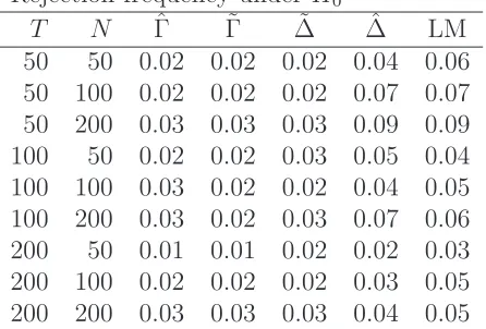
The finite sample properties of the proposed test under each of the data generating processes are summarized in Tables 1–3. Each column reports the rejection frequency (= the number of rejections/2,000) under the null H0 and alternative H1. Table 1
provides the results for the first data generating process, and gives the size and power for a wide range ofN andT. The results for ˆ∆ and ˜∆ are in line with those of Pesaran and Yamagata (2008). Furthermore, the LM results are in line with those of Su and Chen (2013).
Table 1 suggests that the level of our test behaves reasonably well as the size of the panel increases N, T → ∞. When the null hypothesis does not hold, Table 1 suggests our test statistics ˆΓ and ˜Γ have higher power than those of ˆ∆ and ˜∆ under small T
and N.
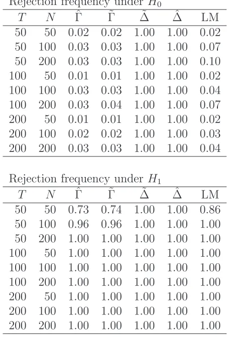
However, we can see the clear advantages of our testing procedure in Table 2. Under the null, Pesaran and Yamagata’s (2008) testing procedure rejects the null in almost all cases. In contrast, our testing procedure has nice size control and power for all combinations of N and T. This difference arises because xit and the factor structure are correlated in the second data generating process. Our test permits this correlation. Su and Chen’s (2013) procedure works well in general. There is, however, a tendency of size distortion when N is relatively large with respect to T, for example, T = 50 and N = 200. A possible reason is that their test imposes the following conditions:
N3/4
/T →0 andT2/3
/N →0 asN, T → ∞. In general, these conditions are sufficient, and they are not necessary. Nevertheless, they imply a relatively narrow band between
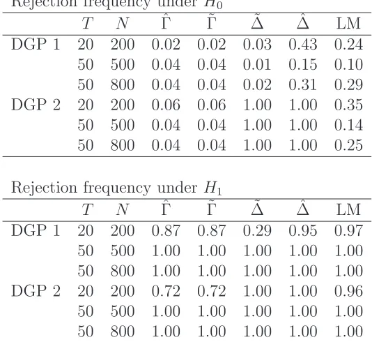
N andT. To verify this, we further compared the size and power of all tests under large N. Under much largerN relative toT, the finite sample properties of the proposed test are summarized in Table 3. Under the second data generating process with (N, T) = (200,20), the finite sample rejection frequencies at an α = 5% nominal level for our test were 0.06 under the null H0 and 0.72 under the alternativeH1. However, those of
Su and Chen’s (2013) test are 0.35 under the null H0 and 0.96 under the alternative
H1. It can be seen that our proposed test still provides correct size, while a size
the relationship betweenN and T. Similar observations can be made for Pesaran and Yamagata’s (2008) ˆ∆ test statistic. As ˜∆ needs the weaker condition √N /T2
→ 0, the ˜∆ procedure has nice size control under the first DGP, but not under the second DGP, as before. Our test continues to work well under much larger N than T.
5
Conclusion
In this paper we examined the problem of testing slope homogeneity in a high-dimensional panel data model. We developed testing procedures based on the Swamy’s (1970) test principle. Our testing procedure allows cross-sectional dependence as well as the de-pendence between the predictors and unobservable factor structures. Monte Carlo experiments suggest that the proposed method is a useful testing procedure for detect-ing slope homogeneity in high-dimensional panel data in which both the time dimension and the cross-sectional dimension are large.
References
[1] Ando, T. & Bai, J. (2014) Asset pricing with a general multifactor structure.
Journal of Financial Econometrics, forthcoming.
[2] Bai, J. (2009) Panel data models with interactive fixed effects. Econometrica 77, 1229–1279.
[3] Bai, J. & Ng, S. (2002) Determining the number of factors in approximate factor models. Econometrica 70, 191–221.
[4] Blomquist, J. & Westerlund, J. (2013) Testing slope homogeneity in large panels with serial correlation.Economics Letters 121, 374–378
[5] Carhart, M. M. (1997) On persistence in mutual fund performance. Journal of Finance52, 57–82.
[6] Connor, G. & Korajczyk, R. (1986) Performance measurement with the arbitrage pricing theory: a new framework for analysis.Journal of Financial Economics15, 3730–3794.
[7] Fama, E. & French, K. (1992) The cross-section of expected stock returns.Journal of Finance 47, 427–465.
[9] Pesaran, M. H. & Yamagata, T. (2008) Testing slope homogeneity in large panels.
Journal of Econometrics 142, 50–93.
[10] Pesaran, H., Smith, R. & Im, K. S. (1996) Dynamic linear models for heteroge-nous panels. In: Matyas, L. & Sevestre, P. (Eds.), Econometrics of Panel Data: A Handbook of the Theory with Applications, second revised edition. Kluwer Aca-demic Publishers, Dordrecht, 145–195.
[11] Phillips, P. C. B. & Sul, D. (2003) Dynamic panel estimation and homogeneity testing under cross section dependence. Econometrics Journal 6, 217–259.
[12] Sharpe, W.F. (1964) Capital Asset Prices: A Theory of Market Equilibrium under Conditions of Risk.Journal of Finance. 19:3, 425-442.
[13] Song, M. (2013) Essays on Large Panel Data Analysis. Ph.D. Thesis, Columbia University.
[14] Su, L. & Chen, Q. (2013) Testing homogeneity in panel data models with inter-active fixed effects. Econometric Theory 29, 1079–1135
[15] Swamy, P. A. V. B. (1970). Efficient inference in a random coefficient regression model. Econometrica 38, 311–323.
Appendix 1: Proof of Theorem 1. Let ˆβi be obtained by minimizing the least-squares objective function in (7). Let Sii = (Xi′MF0Xi)/T, Lij = aij(X′
iMF0Xj)/T
with aij =λ0j
′
(Λ0′
Λ0
/N)−1
λ0j and ζi =X′
iMF0εi/
√
T. Song (2013) rigorously showed that under √T /N →0,
√
T( ˆβi−β0i) =S−1
ii ζi+S−
1 ii 1 N N X j=1 Lij √
T( ˆβj−β0j) +op(1), i= 1, ..., N,
which implies √ T ˆ
β1−β 0 1
ˆ
β2−β 0 2
... ˆ
βN −β0N
=
S−1 11
S22−1
. ..
SN N−1
ζ1 ζ2 ... ζN +1 N
S−1 11
S22−1
. ..
SN N−1
L11 L12 · · · L1N
L21 L22 . .. L2N
... . .. ... ...
LN1 LN2 · · · LN N
√
T( ˆβ1−β 0 1)
√
T( ˆβ2−β 0 2)
...
√
T( ˆβN −β0N)
We can express the above formula as
√
T( ˆβ−β0) =S−1
ζ+ 1
NS
−1
L√T( ˆβ−β0) +op(1), (11)
where ˆβ′ = ( ˆβ′1, ...,βˆ
′
N), β
0′
= (β01
′
, ...,β0N′), ζ′ = (ζ1′, ...,ζ′N), S is an N p×N p block
diagonal matrix with ith block Sii, and L is an N p×N p matrix with ij-th block Lij.
Let Ω be the variance–covariance matrix of ζ, that is block diagonal matrix,
Ω = Ω1 Ω2 . .. ΩN , (12)
where Ωi is the variance–covariance matrix of ζi.
From (11), we then have
Ω−1/2
µ
S− 1
NL
¶√
T( ˆβ−β0) = Ω−1/2ζ +op(1),
which implies
T( ˆβ−β0)′
µ
S− 1
NL
′
Ω−1
µ
S− 1
NL
( ˆβ−β0) =ζ′Ω−1
ζ +op(1).
From Assumption (E), ζ′Ω−1
ζ in the last line asymptotically follows a chi-squared distribution withN pdegrees of freedom. Because the noise terms are cross-sectionally independent as in Assumption (C), by the central limit theorem, we have
ζ′Ω−1
ζ−N p
√
2N p →N(0,1).
It can be shown that replacing β0 by ¯β1N, and the unknown elements in S, L, and
Ω by their estimators, the same asymptotic representation holds. This completes the proof of Theorem 1.
Appendix 2: Proof of (10). The test statistic ˆΓ is derived by correcting bias for the whole system (joint bias). If we correct the bias for each individual parameter ˆβi, then using
1
NS
−1
ii Lii=
1
NaiiIp =λ
0
i
′
(Λ0′
Λ0
)−1
λ0iIp,
we have
√
T( ˆβi−β0i) = Sii−1ζi+ 1
Naii
√
T( ˆβi−β0i) +op(1).
The reason that this approximation works is that the weighted average of ( ˆβj −β0j) for j 6=i,
S−1
ii
1
N
X
j6=i
Lij
√
is of small magnitude, and is also uncorrelated with the leading termζi. This leads to
Sii
√
T( ˆβi−β0i)(1−aii/N) = ζi+op(1),
or
Ω−i 1/2Sii
√
T( ˆβi−β0i)(1−aii/N) = Ω−
1/2
i ζi+op(1).
We then have
T( ˆβi−β0i)′SiiΩ−1Sii( ˆβi−β
0
i)(1−aii/N)2 =ζ′iΩ−
1
i ζi+op(1),
Table 1: Finite sample properties of the proposed test under the first data generating process. Each column reports the rejection frequency under the nullH0 and alternative H1. Critical level is set asα = 5%. ˆΓ: the proposed test statistic in (8), ˜Γ: the proposed
test statistic in (10), ˆ∆: the test procedure of Pesaran and Yamagata (2008) in (2), ˜∆: the test procedure of Pesaran and Yamagata (2008) in (3) and LM: the residual-based Lagrangian Multiplier test of Su and Chen (2013) in (4).
Rejection frequency under H0
T N Γˆ Γ˜ ∆˜ ∆ˆ LM 50 50 0.02 0.02 0.02 0.04 0.06 50 100 0.02 0.02 0.02 0.07 0.07 50 200 0.03 0.03 0.03 0.09 0.09 100 50 0.02 0.02 0.03 0.05 0.04 100 100 0.03 0.02 0.02 0.04 0.05 100 200 0.03 0.02 0.03 0.07 0.06 200 50 0.01 0.01 0.02 0.02 0.03 200 100 0.02 0.02 0.02 0.03 0.05 200 200 0.03 0.03 0.03 0.04 0.05
Rejection frequency under H1
Table 2: Finite sample properties of the proposed test under the second data generating process. Each column reports the rejection frequency under the nullH0 and alternative H1. Critical level is set asα = 5%. ˆΓ: the proposed test statistic in (8), ˜Γ: the proposed
test statistic in (10), ˆ∆: the test procedure of Pesaran and Yamagata (2008) in (2), ˜∆: the test procedure of Pesaran and Yamagata (2008) in (3) and LM: the residual-based Lagrangian Multiplier test of Su and Chen (2013) in (4).
Rejection frequency under H0
T N Γˆ Γ˜ ∆˜ ∆ˆ LM 50 50 0.02 0.02 1.00 1.00 0.02 50 100 0.03 0.03 1.00 1.00 0.07 50 200 0.03 0.03 1.00 1.00 0.10 100 50 0.01 0.01 1.00 1.00 0.02 100 100 0.03 0.03 1.00 1.00 0.04 100 200 0.03 0.04 1.00 1.00 0.07 200 50 0.01 0.01 1.00 1.00 0.02 200 100 0.02 0.02 1.00 1.00 0.03 200 200 0.03 0.03 1.00 1.00 0.04
Rejection frequency under H1
Table 3: Finite sample properties of the proposed test under large number of units N
compared with the length of time seriesT. Each column reports the rejection frequency under the null H0 and alternativeH1. Critical level is set asα = 5%. ˆΓ: the proposed
test statistic in (8), ˜Γ: the proposed test statistic in (10), ˆ∆: the test procedure of Pesaran and Yamagata (2008) in (2), ˜∆: the test procedure of Pesaran and Yamagata (2008) in (3) and LM: the residual-based Lagrangian Multiplier test of Su and Chen (2013) in (4).
Rejection frequency under H0
T N Γˆ Γ˜ ∆˜ ∆ˆ LM DGP 1 20 200 0.02 0.02 0.03 0.43 0.24 50 500 0.04 0.04 0.01 0.15 0.10 50 800 0.04 0.04 0.02 0.31 0.29 DGP 2 20 200 0.06 0.06 1.00 1.00 0.35 50 500 0.04 0.04 1.00 1.00 0.14 50 800 0.04 0.04 1.00 1.00 0.25
Rejection frequency under H1