Structure Learning in Weighted Languages

Structure Learning in Weighted Languages

Andr´as Kornai, Attila Zs´eder, G´abor Recski HAS Computer and Automation Research Institute

H-1111 Kende u 13-17, Budapest

{kornai,zseder,recski}@sztaki.mta.hu

Abstract

We present Minimum Description Length techniques for learning the structure of weighted languages. MDL is already widely used both for segmentation and classification tasks, and here we show it can be used to formalize further important tools in the descriptive linguists’ toolbox, including the distinction between acciden-tal and systematic gaps in the data, the de-tection of ambiguity, the selective discard-ing of data, and the mergdiscard-ing of categories.

Introduction

The Minimum Description Length (MDL, see Ris-sanen 1978) framework is primarily about data compression: if we are given some data D, our goal is to find a modelM, and a correction term E, such that the model output and the correction term together describe the data, and transmitting M and E takes fewer bits than transmitting any competingM0andE0.

From the very beginning, starting with P¯an.ini, linguists have put a premium on brevity. The hope is that the shortest theory is the best theory (see Vitanyi and Li 2000), at least if we are willing to posit a theory of Universal Grammar (UG) that will let us specifyMbriefly, since we can assume UG to be amortized over many languages.

In this paper we study the problem of com-pressing weighted languages by presenting them via weighted finite state automata (WFSA). The theoretical approach we discuss here has a long history: the founding paper of Kolmogorov com-plexity, Solomonoff (1964), already studied the problem of inferring a grammar from data, and Gr¨unwald (1996) uses MDL to infer CFGs from corpora, there conceived of as long strings over a finite alphabet. It is fair to say that this theory has not had much impact on computational practice,

where grammatical inference is dominated by the standard n-gram based language modeling meth-ods, see Jelinek (1997) for an excellent summary of the basic ideas and techniques, most of which are still in wide use.

While the two approaches may coincide in cer-tain cases (see Gr¨unwald 1996), and in theory n-gram models are just a special case of the general WFSA, in practice they are divided by a funda-mental difference in modeling unseen data. From an engineering standpoint, Church et al (2007) are entirely right in saying:

No matter how much data we have, we never have enough. Nothing has zero probability.

Linguists, starting perhaps with Chomsky (1965), draw a bright line between accidentallyand sys-tematicallymissing data, and would prefer to re-strict backoff techniques to the accidental gaps. The distinction is often lost in applied work, be-cause the models need to be built in a noisy envi-ronment, where frequent typos like*tehand simi-lar performance errors can easily overwhelm gen-uine items likeboisterousormopedsby an order of magnitude or even more. In the eyes of many linguists, this observation alone is sufficient to rob probabilistic models of grammatical content, since this makes it impossible to define a single thresh-old g such that all and only strings with weight greater thangare grammatical.

as Hidden Markov Models (HMMs) and proba-bilistic context-free grammars (PCFGs) with very many parameters, and stops adding more only when compressing the memory footprint is of paramount importance. As (Church et al., 2007) notes, applications like the contextual speller of Microsoft Office simply could not ship without keeping the language model within reasonable size limits. In such cases, we are quite willing to trade inEfor gains in the sizeM ofM, and con-siderations of optimizing the sum of the two are simply irrelevant.

In contrast, our strategy is to search for model which measures bothMandE in bits, and opti-mizes the sumM +E, not because we put such a premium on data compression, but rather be-cause we follow in P¯an.ini’s footsteps. Our goal is finding structural models capable of distinguish-ing structurally excluded (ungrammatical) strdistinguish-ings likefuriously sleep ideas green colorlessfrom low probability but grammatical strings likecolorless green ideas sleep furiously (Pereira, 2000). For this more ambitious goal comparing models with different number of parameters is a key issue, and this is precisely where MDL is helpful.

The rest of this Introduction provides the basic definitions, notation, and terminology, all fairly standard except for the use of Moore rather than Mealy machines – the significance of this choice will be discussed in Section 2. In Section 1 we bring a fundamental idea of signal process-ing, quantization error, to bear on the problem of model selection, illustrating the issue on a real example, the proquant system of Hungarian. In Section 2 we show how one of the most power-ful tools at disposal of the linguist,ambiguity, can be detected by MDL, bringing another standard idea, signal to noise ratio to bear. In Section 3 we discuss another real example, Hungarian mor-photactics, and show that two methods widely (but shamefacedly) used in practice, discarding data and merging descriptive categories, can be used on a principled basis within MDL. Our goal is to show that by consistent application of MDL principles we can automatically set up the kind of models that linguists would set up. Ultimately, both man and machine work toward the same goal, optimization of grammar elegance or, what is the same, brevity.

Definition 1. Given some finite alphabet Σ, a weighted languagepover this alphabet is defined

as a mappingp: Σ∗→_Rtaking non-negative val-ues such thatP

α∈Σ∗p(α) = 1. This is less gen-eral than the standard notion of noncommutative power series with weights taken in arbitrary semir-ings (Eilenberg 1974, Salomaa 1978) but will suf-fice here. The stringset{α|p(α)>0}is called the supportofpand will be denoted byS(p).

Definition 2. Given two weighted languages p and q, we say the Kullback-Leibler (KL) approximation error Q of q relative to p is

P

α∈S(q)p(α) log(p(α)/q(α)). Theentropy ofp

is defined as−P

α∈S(p)p(α) log(p(α)).

Definition 3. A WFSAMis defined by a square transition matrix M whose elementmij give the probability of transition from stateito statej, an emission lisththat gives a stringhi∈Σ∗for each i6= 0, and an acceptance vector~awhosei-th com-ponent is 1 ifiis an accepting state and 0 other-wise. There is a unique initial state which starts the state numbering at 0, and we permit states with empty outputs. Rows ofM must sum to 1. Thus we have defined WFSA as normalized probability-weighted nondeterministic Moore machines.

Definition 4. The weight a WFSA assigns to a generation path is the product of the weights on the edges traversed, and the weight it assigns to a stringα is the sum of the weights assigned to all paths that generateα.

1 Quantization error

The notions of quantization error and quantiza-tion noise, while well known in the signal pro-cessing literature (for a monographic treatment, see Widrow and Koll´ar 2008), and widely used in speech processing (Makhoul et al., 1985), have had little impact on language processing. Yet MDL description of even the simplest weighted language brings up a significant problem that can-not be addressed without approximation.

As long as the weights themselves are treated as information objects of arbitrary capacity, there is no way out of this conundrum (de Leeuw 1956). On the other hand, the weighted languages we en-counter in practice are generally abstracted from gigaword or smaller corpora, and as such their in-herent precision is less than 32 bits. For weighted languages with finite support (corpora and lan-guage models without smoothing) p is simply a list containing strings and probabilities. The cost of transmitting this list comes from two sources: the cost of transmitting the probabilities, and the cost of transmitting the strings. As a first approx-imation, let us assume the two are independent, a matter we shall return to in Section 2.

We begin by investigating the inherent cost/error tradeoff of transmitting a discrete probability distribution {pj|1 ≤ j ≤ k} by uniform quantization tobbits. We divide the unit interval inn = 2b _{equal parts. For our theorems} we will use a value b large enough so that we have pj ≥ 2−(b−2) for all j, leaving at least the first 4 bins empty. Usually 32 bits suffice for this, and as we shall see shortly, often a lot fewer are truly needed, though standard modeling tools like SRILM often use 64-bit quantities. For each probability, Alice sends b bits (the bin number). Bob, who knowsb, reconstructs a value based on the center of the bin.

Since this process does not guarantee that the reconstructed values sum to 1, Bob takes the ad-ditional step of renormalizing these values: if

P

qi = r, he will use q = qi/r instead of the qithat were transmitted by Alice. Whenbis large, thepi will be distributed uniformly mod2−b. In this case, the expected valuesE(pi−qi)are zero for alli, so E(P

qi) = P

E(qi) = P

E(pi) = E(P

pi) = 1or, in other words,E(r) = 1. Since Var(r −1) = P

iVar(pi −qi) = k/12n2 is on the order1/n2, in the following estimate we can safely ignore the effects of renormalization. By Definition 2, the KL approximation error is

Q= n−1

X

i=0

X

i/n≤pj≤(i+1)/n

pj∆(pij) (1)

where ∆(pi

j) = log(2npj/(2i + 1)) is the dif-ference between the logarithms of the actual pj and the centerpoint of the interval[i/n,(i+ 1)/n) wherepj falls. In absolute value, this is maximal whenpj is at the lower end of this interval, where ∆(pi_j) islog(2i₂+1_i ). Using the standard estimate

log(1 +x) ≤ x this will be less than ₂1_i ≤ 1/8 sincei≥ 4. Since the ∆(pi_j)are now estimated uniformly, and thepjsum to 1, we obtain

Theorem 1. The approximation errorQnof uni-form quantization intonbins[i/n,(i+1)/n)such that the first 4 bins are empty satisfies

Qn≤ 1

8 log 2 ∼0.18 (2)

bits independent ofn(the computation was in base erather than base 2, hence the factorlog 2). With growingnthe number of bins that remain empty will grow, and the estimate ₂1_i of ∆ can be im-proved accordingly.

Theorem 1 of course gives just an upper bound, and a rather crude one, the expected value ofQn is considerably less. Instead of using the max value ∆(pi_j) we can consider the expected abso-lute value, which islog(1 +₂1_i)/n, so equation (2) could be reformulated as

E(Qn)≤ 1

8nlog 2 (3)

It is evident from the foregoing that the crux of the matter are the smallpi values, and at any rate, there can only be a handful of relatively large val-ues, since the sum is 1. Experience shows that probabilities obtained from corpora span many or-ders of magnitude, which justifies the use of a log scale. Instead of the simple uniform quantization of Theorem 1, we will use a two-parameter quan-tization scheme, whereby firstlogpj are cut off at −C, and the rest, which are on the(−C,0) inter-val, are sorted inn= 2b _{bins ‘b-bit quantization’.}

In effect, all probabilities below e−C are as-sumed to be below measurement precision, and the log of the rest are uniformly quantized. We experimented with two simple techniques: repre-senting the class(−∞,−C)with a very low fixed value (10−50) or with one set to e−2C based on the parameter C of the encoding. As there was no appreciable difference (which is not surprising givenlimx→0xlogx = 0), from here on we

∅ a ak´ar b´ar egyvala m´as m´asvala minden se vala

h´any 72383 9502 2432 55 21 4584

hogy 7781539 213687 3173 1839 4570 123 4138 31873

hol 117231 399052 1037 9845 16066 16009 20521 34081

honnan 24777 18628 296 1205 2482 1321 627 4274

honn´et 1598 1197 12 25 78 33 23 236

hov´a 17589 21073 486 1753 1 5073 1 1859 2249 3966

hova 17360 10591 309 1166 1788 1381 2105 3036

ki 1309618 1464744 3933 60923 884 814 308508 165230 221175

meddig 11879 8171 189 225 74 252

mely 761277 1586913 166 74262 3 4 40601

melyik 68051 47564 1996 34477 2 939 48274

mennyi 76429 25805 657 1415 517 96184

mi 1626013 1303820 6500 52480 1337 161 275773 355690

mi´ert 251120 20672 58 205 4 1810 13552

mikor 173652 555325 679 33516 15892 11288 206 18235

milyen 343643 38921 8217 68033 1618 1 55603 81155

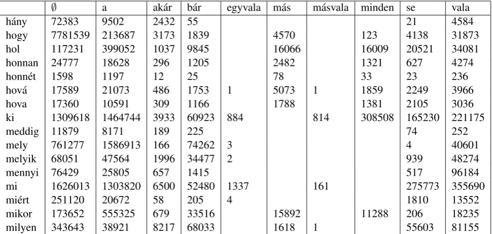
Table 1: Frequencies of proquants in the Hungarian Webcorpus

generally 1-5% of the probability mass, to un-seen events, and use calculated numbers, instead of measured values, to smooth the distribution. Unfortunately, the engineering philosophy behind the various backoff schemes (which often utilize MDL stopping criteria both in speech and lan-guage modeling, see e.g. Shinoda and Watanabe 2000, Seymore and Rosenfeld 1996) is diametri-cally opposed to the the method of inquiry pre-ferred by linguists, whose primary interest is with generalization, i.e. with models that make falsifi-able predictions, rather than furnishing descriptive statistics. In particular, negative generalizations, that something is forbidden by some rule of gram-mar, are just as interesting from their standpoint as positive generalizations. But how do we express a negative generalization?

Definition 5.A string will be deemed ungrammat-icalor structurally excluded iff every generation path includes at least one zero weight in the above sense.

If scores from different sources are multiplied together, the use of zero weights as markers of ungrammaticality is implicit in the semantics of WFSA.1 Still, there are significant difficulties in implementing the idea. If we want to maintain the commonsensical assumption that *teh is not a word (has zero unigram weight) and also ac-count for the data that makes it the 34,174th most common string in English text, we will need to

1_{We owe this observation to an anonymous MOL referee.}

model typos. Once we learn that the log price of the /the/teh/ substitution is about -9.8, we can pre-dict not just the frequency ofteh, but also those ofweatehr, otehr, tehy, tehre, tehft, and so forth, without adding these to the lexicon. Since such a model is based on computed frequencies of letter substitution and exchange rather than on the typos directly, the engineer has to give up the enterprise of building the entire language model in a single sweep directly on the data.

At the same time, the linguist has to give up the attractive simplicity of ‘zero weight iff un-grammatical’: the misspelling model will assign a low but nonzero weight to everything, and if this model is compiled together with a unigram model that contains only grammatical words, the simple world-view of Definition 5 will no longer work. Rather, we will have to say that it is zero weight in thegrammaticalsubautomaton (visible only prior to getting compiled together with the se-mantic, spelling, stylistic, and possibly other sub-automata) that defines grammaticality. We have to build an explicit noise model to make sense of the raw data, but this is not particularly surprising from the perspective of other sciences like astron-omy where noise reduction is common practice.

these points in Sections 2 and 3, we need to as-similate another piece of computational practice, the use of log probabilities. When quantization is uniform on the log scale, the expected value of the binning error is no longer zero, given our assump-tion of uniformity on the linear scale, but rather

−Clog_ni

Z

−Clogi+1_n

ex−e−Ci+0n.5dx∼C3/8n3 (4)

which yields an expectedr ∼kC3/8n3, still neg-ligible compared to the bound given in Theorem 2, which is obtained by methods similar to those used above.

Theorem 2. For C, n sufficiently large for the first 4 bins to remain empty, the approximation errorLC_n of log-uniform quantization with cutoff −C into n = 2b bins[−C(i+ 1)/n,−Ci/n)is bounded by

LC_n ≤ C

2nlog 2 (5)

and the expected value E(LC_n) is bounded by C2/4n2log 2.

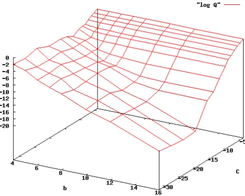
Figure 1:Error of log-scale uniform quantization

Let us see on an example how these error bounds compare to values obtained numerically. Our first example will explore what we will call, for want of a better name, the proquant system of Hungarian that covers both pro-forms (pro-nouns, proadjectives, proadverbials) and quan-tifiers. Given the prefixes a-, minden-, vala-, egyvala-, m´asvala-, se-, ak´ar-, m´as-, b´ar- and

zero, and suffixes -ki, -mi, -hol, -hogy, -hova, etc. we can create forms such as valaki ‘some-one’, valami‘something’, ak´arki‘anyone’, sehol ‘nowhere’ and so on. Clearly, many of what we call prefixes and suffixes could be analyzed fur-ther, e.g.m´asvalaasm´as+vala, but we don’t want to prejudge the issue by presenting a maximally detailed analysis.

In a corpus of over 40 million sentences (Hun-garian Webcorpus, Hal´acsy et al. 2004) we ob-served the frequencies in Table 1. Many of these proquant forms take inflectional suffixes (case, number, etc.), and the numbers presented here al-ready include these, so that the 814 occurrences of m´asvalaki include forms like m´asvalakivel ‘with someone else’, m´asvalakinek ‘to someone else’ etc. If we think of the (stemmed) Hungarian vo-cabulary as a weighted language h, the set of prefixes (suffixes) as an unweighted language Pre (resp. Suff), the data is a sample from S(h)∩ Pre·Suff with the weights renormalized. Alto-gether, we have 121 nonzero values plus 39 ze-ros, the entropy of the distribution isH = 3.677. Figure 1 plots the log of the observed quantiza-tion noise as a funcquantiza-tion of the number of bitsband the cutoff−C. Notice that onceC is sufficiently large, no further gains are made by increasing it further. As expected from Theorem 2, the log of the error is roughly linear inb = log₂n(the ob-served values are of course better than the bounds).

Definition 6. The inherent noise of a dataset D is the KL approximation error between a random subsample and its complement.

Ideally, we would want to compare another sam-pleD0 toD, but in many cases launching a com-parable data collection effort is simply not feasi-ble, and we must content ourselves with the sim-ple procedure suggested by this definition. By ran-domly cutting the 40m sentence corpus on which the proquant dataset is based in 10m sentence parts and computing the KL divergence between any two, we obtain numbers in the 7-8·10−5 range, which means it makes little sense to approximate Dwith better precision than10−5. How to handle the singular cases when some qj becomes 0 (as happens with half of the hapaxes when we cut the sample in two) is an issue we defer to Section 3.

a final state, and a separate Mealy arc (or Moore state) for each of the 121 nonzero observations al-ready generate a weighted language within the in-herent noise of the data at 10 bits, where the KL divergence is at8·10−6. At 12 bits, the divergence is below1.4·10−6, and at 16 bits, below5·10−9. As we shall see in the next Section, the MDL size of these models, between 2k and 7k bits, is domi-nated by factors unrelated to the precisionbof the encoding.

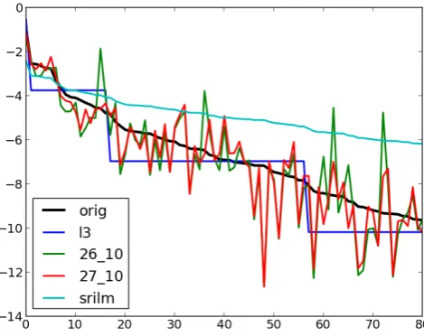
Figure 2:Model fit to observed probabilities

Figure 2 shows the 80 largest observed proquant probabilities (in black) in descending order, and the probabilities of the same strings as computed from several models. The 10 and 12-bit list au-tomata are not plotted, as the computed values are graphically indistinguishable from the observed values, the rest will be discussed in the text.

2 Detecting ambiguity

Before turning to the actual MDL learning pro-cess, let us summarize what we have for the Hun-garian proquant system so far. We have a weighted language of about 120 strings. When transmit-ting a weighted automaton, Alice is sending not strings and weights, but rather weight-labeled arcs and string-labeled states of a WFSA. In Defini-tion 3 we used Moore machines, but in the liter-ature Mealy automata, where inputs/outputs and weights are both tied to arcs are more common (see e.g. Mohri 2009). The rationale for preferring Moore over Mealy in the MDL context is that no gains can be obtained from joint compression of strings and probabilities (even though Mealy ma-chines couple the two), while sharing of strings

has very significant impact on MDL length, as we shall see shortly. For the simple ‘list’ automata this means adding extra states in the middle of a Mealy arc, and we need to take some precautions to guarantee that the representation is just as com-pact as it would be for a Mealy machine.

Let us now see in some detail how compact these encodings can get. Withsstates, andbbits for probability, an arc requires 2 log₂s+b bits. However, Bob can reasonably assume that Alice is only sending trimmed machines, with states that cannot be reached from the initial state or with no path to an accepting state already removed. There-fore, if Bob sees a state with no outbound path he supplies an outgoing arc, with probability 1, to the final state – such arcs need not be sent by Al-ice to begin with. Similarly, Bob can assume that all states except for the last one are non-accepting, and Alice will transmit information only to over-ride this default when needed.

As for emissions, in a Moore machine each state emits a string (but no guarantees that different states emit different strings), so Alice needs to en-code the strings somehow. If we assume that there is a character table shared between Alice and Bob, e.g. the character frequencies of Hungarian, with entropyH, encoding a stringαcosts simply|α|H bits. (We could take this also to be a case of trans-mitting a weighted language, but we assume that the cost of transmitting this language can be amor-tized over many WFSA that deal with Hungarian.)

b l M cs ca KL Hq

1 121 5210 4306 904 2.1883 6.833 2 121 5386 4306 1080 1.1207 3.487 3 121 5507 4306 1201 0.268 2.889 4 121 5628 4306 1322 0.041436 4.044 5 121 5749 4306 1443 0.016117 3.424 6 121 5870 4306 1564 0.002409 3.667 7 121 5991 4306 1685 0.000676 3.653 8 121 6112 4306 1806 0.000288 3.647 9 121 6233 4306 1927 5.905e-5 3.681 10 121 6354 4306 2048 8.003e-6 3.678 11 121 6475 4306 2169 3.999e-6 3.678 12 121 6596 4306 2290 1.387e-6 3.678 16 121 7080 4306 2774 4.660e-9 3.676

Table 2: List models with character-based string encoding

number of trainable parameters (weights associ-ated to arcs),cais the cost of transmitting the arcs. Note that this is less thanl(b+2 log₂s), because of the redundancy assumptions shared by Alice and Bob. cs is the cost of transmitting the emissions, and the total model cost is M = ca +cs. We would, ideally, also need to add toM a dozen bits or so to encode the major parameters of the cod-ing scheme itself, such as the valuesb = 10and C = 20, but these turn out to be negligible com-pared to the basic cost. Also, these major param-eters are shared across the alternatives we com-pare, so whatever we do to minimizeM will not be affected by uniformly adding (or uniformly ig-noring) this constant cost. KL gives the KL di-vergence between the model and the training data. This measures the expected extra message length per arc weight, so that the error residual E is k times this value, wherekis the number of values being modeled. We emphasize that k = l only in the listing format, where all values are treated as independent – in the ‘hub’ model we shall dis-cuss shortly lis only 26 (10 prefix and 16 suffix weights) butkis still 121.

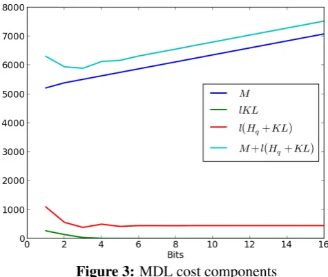
The main components of the total MDL cost, M,l·KL,l(KL+Hq), and the totalM+l(KL+ Hq)are plotted on Figure 3.

Figure 3:MDL cost components

All models with b ≥ 10 are within the inter-nal noise of the data, and it takes over 6kb to de-scribe such a model. However, the bulk of these bits come from encoding the output strings char-acter by charchar-acter – if we assume that Alice and Bob share a morpheme table, the results improve a great deal, by over 3,600 bits. If the system rec-ognizes what we already anticipated in Table 1,

that each string can be expressed as the concate-nation of a prefix and suffix, encoding the strings becomes drastically cheaper. Using MDL for seg-mentation is a well-explored area (see in particular Goldsmith 2001, Creutz and Lagus 2002, 2005), and we are satisfied by pointing out that using the morphemes in the first row and column of Table 1 we drastically reduce cs, to about 708 bits, below the cost ca of encoding the probabil-ities. The 3-bit list model providing the MDL op-timum (dark blue in Figure 2) requires 1,900 bits with this string encoding, and is noticeably better than the SRILM bigram/trigram (turquoise) which takes around 12kb.

By encoding the emissions in a more clever fashion, we have not changed the structure of the model: the same states are still linked by the same arcs carrying the same probabilities, it is just the state labels that are now encoded differently. When expressed as a Mealy automaton, a listing of probabilities corresponds to a two-state WFSA with as many arcs as we have list elements (in our case, 121), while the arrangement of Table 1 is suggestive of a different model, one with 10 prefix arcs from the initial state to a central ‘hub’ state, and 16 suffix arcs from this hub to the final state.

We have trained such ‘hub’ models using KL, Euclidean (L2), and absolute value (L1)

minimiza-tion techniques. Of these, direct minimizaminimiza-tion of KL divergence works best, obtaining 0.325 bits at b= 10, and 0.298 atb= 12(red and green in Fig-ure 2). While the difference, about 0.027 bits, is still perceptible compared to the noise level, with a signal to noise ratio (SNR) of 8 dB, it simply does not amortize over the 26 model probabilities we need to encode. Adding 2 bits for encoding one value requires a total of adding 52 bits to our spec-ification ofM, while the gain of the error residual E, computed over the 121 observed values, is just 2.074 bits. In short, there is not much to be gained by going from 10 to 12 bits, and we need to look elsewhere for further compression.

Definition 7. For a weighted languagepa model transformX islearnable in principle (LIP) if (i) both M and X(M) are part of the hypothesis space and (ii) the total MDL cost of describingp byX(M)is significantly below that of describing pbyM.

bill may not be feasible. The difference between LIP and practical MDL learnability is precisely the difference between existence proofs and construc-tive proofs. Our interest here is with the former: our goal is to demonstrate that structurally sound models are LIP. So far, we have seen that struc-turally valid segmentations can be effectively ob-tained by MDL. Our next task is to show that am-biguityis LIP.

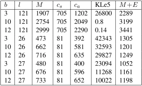
As linguists, we know that the weakest point of the hub model is thathogy, accounting for almost 40% of the data, is not just a proquant ‘how’ but also a subordinating conjunction ‘that’. To encode this ambiguity, we add another arc emittinghogy directly. Table 3 compares list models (lines 1-3, emissions encoded over morphemes rather than characters), simple hub models (lines 4-6), and hub models with this extra arc (lines 7-9).

b l M cs ca KLe5 M+E

3 121 1907 705 1202 26800 2289 10 121 2754 705 2049 0.8 3199 12 121 2999 705 2290 0.14 3441 3 26 473 81 392 42343 1305 10 26 662 81 581 32593 1201 12 26 716 81 635 29827 1249 3 27 480 81 400 23094 1052 10 27 676 81 596 11268 1161 12 27 733 81 652 10022 1198

Table 3: Hub models with/out ambiguoushogy

As can be seen from the table, the best model again takes only 3 bits, but must include the ex-tra parameter for handling the ambiguity ofhogy. To learn this, at least in principle, without relying on the human knowledge that drove the heuristic search, consider the leading terms of the KL error. Arranging thepilog(pi/qi)in order of decreasing absolute value we obtain mi 0.0192; minden+ki 0.0175; a+mely 0.0169; mely -0.0147; a+mikor 0.0135;hogy-0.0128; and so forth. Of all the 121 strings we may consider for direct emission, only hogyis worth adding a separate arc for. Further, if we repeat the process, adding a second direct arc never results in sufficient entropy gain compared to addinghogyalone.

To summarize, list models can approximate the original data within its inherent noise level, but incur a very significant MDL cost, even if they use an efficient string encoding because they keep many parameters, see the first three lines of Ta-ble 3 above. The hub models, which build struc-ture similar to the one used in the string encoding,

recognizing prefixes and suffixes for what they are, are far more compact, at 470-730 bits, even though they have a KL error of about .1-.4 bits. Finally, the hub+ambiguity model, with 27 parameters, re-duces the total MDL cost to 1052 bits, less than half of the best list model.

Currently we lack the kind of detailed under-standing of the description length surface over the WFSA×stringencoding space that would let us say with absolute certainty that e.g. the hub model with ambiguous hogy is the global mini-mum, and we cannot muster the requisite com-putational power to exhaustively search the space of all WFSA with 27 arcs or less. Further gains could quite possibly made with even cruder quan-tization, e.g. to n = 6 levels (powers of 2 are convenient, but not essential for the model), or by bringing in non-uniform quantization.

On the one hand, we are virtually certain that the only encoding of emissions worth studying is the morpheme-based one, since the economy brought by this is tremendous, 3,600 bits over the proquants alone, and no doubt further gains else-where, as we extend the scope to other words that contain the same morphemes – in this regard, our findings simply confirm what Goldsmith, Creutz, Lagus, and others have already demonstrated. On the other hand, finding the right segmentation is only the first step, we also need a good model of the tactics. As we said at the beginning, the en-coding of arcs and probabilities can to a signifi-cant extent be independent of the encoding of the emissions. Here the remarkable fact is that a bet-ter emission model could to a large extent drive the search for structuring the WFSA itself.

Given a segmentation of a stringα=α1α2, the

hypothesis space includes both a single arc from somer to some twhere we emit α, or the con-catenation of two arcs r → sands → twith s andtemittingα1 andα2respectively. This brings

in a bit of ambiguity in regards to the distribution of the probabilities, for ifαhad weightpthe new arcs could be assigned any valuesp1, p2as long as

p1p2 = p, at least if the sum of outgoing

proba-bilities from sremains 1. If s has no other arcs outgoing than s → t this forces p1 = p, but if

3 Decomposition

For our next example we consider Hungarian stem-internal morphotactics. The Analytic Dic-tionary of Hungarian (Kiss et al 2011) provides, for each stem like beleilleszt ‘fit in’ an analysis like preverb+root+suffix whereinbeleis one of a closed set of Hungarian preverbal particles, illis the root, andesztis a verb-forming suffix. There are six analytic categories: Stem S; sUffix U; Preverb P; rootE; Modified M; and foreIgnI; so that each stem gets mapped on a string over Σ = {S, U, P, E, M, I}. We have two weighted languages: the tYpe-weighted language Y where each string is counted as many times as there are word types corresponding to it (so that e.g. for SUU we have 3,739 stems from ´abr´andozik ‘day-dream’ tozuhanyoz´o‘shower stall’, and the tOken-weightedlanguageO where the same pattern has weight 18,739,068 because these words together appeared that many times in the Hungarian Web-corpus (Hal´acsy et al., 2004).

Since the inherent noise of O is about 0.0474 bits, we are interested in automata that approxi-mate it within this limit. This is easily achieved with HMM-like WFSA that have arcs between any two states, usingb= 11bits or more, the smallest requiring only 781 bits. ForY the inherent noise is less, 0.011 bits, and the complete graph architec-ture, which only has 49 parameters (6 states, plus arcs from an initial state and arcs to a final state) is not capable of getting this close to the data, with the best models, fromb = 11 onwards, remain-ing at KL distance 0.3. The two languages differ quite markedly in other respects as well, as can be seen from the fact that the character entropy ofO is 0.933, that ofY is 1.567. Type frequency is not a good predictor of token frequency: the KL ap-proximation error ofOrelative toY is 2.11 bits.

An important aspect of the MDL calculus is the treatment of the singularities which arise when-ever some of theqi in Definition 2 are 0. In the case at hand, we find both types that are not at-tested in the corpus, and tokens whose type was not listed in the Analytic Dictionary, a situation that would theoretically render it impossible to compute the KL divergence in either direction. In practice, tokens with no dictionary type are either collected in a single ‘unknown’ type or are silently discarded. Both techniques have merit. The catch-all ‘unknown’ type can simply be assumed to fol-low the distribution of the known types, so a model

that captures the data enshrined in the dictionary should, at least in principle, be also ideal for the data not seen by the lexicographer. Surprises may of course lurk in the unseen data, but as long as coverage is high, sayP(unseen)≤0.05, surprises will really be restricted to this 5% of the unseen, or what is the same, will be at orderP2. In general we may consider two distributions{pi} and{qi} as in Definition 2, and compute P = P

qi=0pi,

the proportion ofq-singular data inp.

Theorem 3. The total costL of transmitting an item from the p-distribution is bound by

L≤(1−P)(KL(p, q)+Hq)+P(1+log₂n) (6)

Proof We use, with probability (1−P), the q-based codebook: this will have cost Hq plus the modeling loss KL(p, q). In the remaining cases (probability P) we should use a codebook based on the q-singular portion ofp, but we resort to uni-form coding at costlog₂n, wherenis the number of singular cases. We need to transmit some infor-mation as to which codebook is used: this requires an extraH(P,1−P)≤P bits – collecting these terms gives (6).2

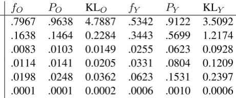
Theorem 3 gives a principled basis for discard-ing data within the MDL framework: whenP is small, the second term of (6) can be absorbed in the noise. To give an example, consider the uni-gram frequencies listed in columnsfO andfY of Table 4. Some letters are quite rare, in particu-lar,I makes up less than 0.06% ofO and 0.013% ofY. Columns KLO and KLY show the KL di-vergence ofOandY from models obtained by by discarding words containing the letter in question, columnsPOandPY show the weight of the strings that are getting discarded.

fO PO KLO fY PY KLY

S .7967 .9638 4.7887 .5342 .9122 3.5092 U .1638 .1464 0.2284 .3443 .5699 1.2174 M .0083 .0103 0.0149 .0255 .0623 0.0928 E .0114 .0141 0.0205 .0331 .0804 0.1209 P .0198 .0248 0.0362 .0623 .1531 0.2397 I .0001 .0001 0.0002 .0006 .0010 0.0006

Table 4: Divergence caused by discarding data

bits; P, I 0.036 bits; and even removing all three ofM, E, Ionly 0.036 bits.

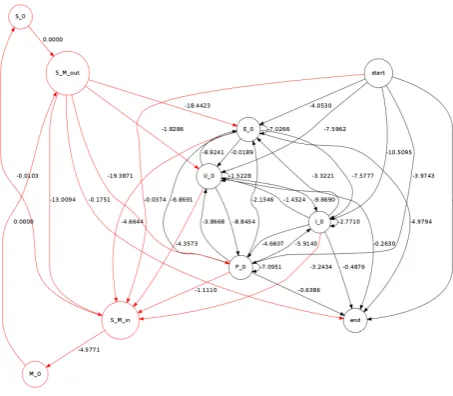
Figure 4:MS merge-split model

In the case of I, again as linguists we under-stand quite well what discarding this data means: we are excluding foreign stems. This is quite jus-tified, not because foreign words like paperback, pacemakerorbaseballare in any way inferior, but because their internal analysis is not transparent to the Hungarian reader (it is telling that the editors of the Analytic Dictionary coded the stem bound-ary inpaper+backbut not inbase+ball).

Discarding M, a category that differs from S only in that the stem undergoes some automatic morphophonological change such as vowel eli-sion, is also a sensible step in that the fundamen-tal morphotactics are not at all affected by these changes, but how is this learnable, even in princi-ple? Here we introduce another model transform calledXY merge-splitcomposed of two steps: first we replace all letters (or strings)XbyY and train a model, and next we split up the emission states ofY in the merged model toX andY-emissions according to the relative proportions of X andY in the original data.

For LIP, the key observation is that models con-structed by XY merge-split have a transmission cost composed of two parts, the length of the smaller merged model (given in black in Figure 2), plus transmitting the pairX, Y and the probability of the split, which is exactly the cost of a single arc, even though the actual split model will have many more arcs (given in red in Figure 4). Once this is taken into account, we can systematically investigate all 6·5 merge-split possibilities. The results confirm the educated linguistic guess quite

remarkably. The best compression rates are ob-tained by merging I with any of the minor cate-gories or, ifI is already discarded or merged in, mergingM into S. The smallestO model before these steps took 781 bits, this is now reduced to 502 bits. If we start by discardingI, and merging MtoSafterwards, this can be reduced to 349 bits. In the end we merge the morphophonologically af-fected forms with the ones not so afaf-fected not be-cause our training as linguists tells us we should do this, but because that is what brevity demands.

4 Conclusions

In this paper we have developed an MDL-based framework for structure detection based on simple notions mostly borrowed from signal processing: quantization noise, inherent noise level, and cut-offs. Standard n-gram models fare rather poorly compared either in size or in model accuracy to the WFSA results obtained here: for example on the morphotactics data a straight SRILM trigram model has over 200 parameters and has KL diver-gence 1.09 bits. Most of the 64 bits per n-gram parameter are wasted (if we assume only 12 bits per parameter, the WFSA we use requires only 49 parameters and gets within 0.03 bits of the ob-served data) and further, the general-purpose back-off scheme built into SRILM just makes matters worse.

Similarly, on the proquant data an SRILM bi-gram model has 175 parameters (including the 26 unigram weights but excluding the backoff weights), yet it is farther from the data at 64 bits resolution than our best 27-parameter model at 3 bits. More important, the bigram structure of the proquant data has to be hand-fed into the standard model, while the MDL approach can discover this, together with other linguistically relevant observa-tions such thathogywas ambiguous.

are LIP, and Universal Grammar is simply a short list of the permissible model transformations in-cluding path duplication for ambiguity, state merg-ing for position class effects, and merge-split for collapsing categories.

Acknowledgments

We thank D´aniel Varga (Prezi) and Viktor Nagy (Prezi) for the first version of the simulated an-nealing WFSA learner. Zs´eder wrote the version used in this study, Recski collected the data and ran the HMM baseline, Kornai advised. The cur-rent version benefited greatly from the remarks of anonymous referees. Work supported by OTKA grants #77476 and #82333.

References

Noam Chomsky and Morris Halle. 1965a. Some con-troversial questions in phonological theory. Journal of Linguistics, 1:97–138.

Kenneth Church, Ted Hart, and Jianfeng Gao. 2007. Compressing trigram language models with Golomb coding. InProceedings of the Joint Conference on Empirical Methods in Natural Language Process-ing and Computational Natural Language LearnProcess-ing, pages 199–207, Prague. ACL.

Mathias Creutz and Krista Lagus. 2002. Unsupervised discovery of morphemes. InProc. 6th SIGPHON, pages 21–30.

Mathias Creutz and Krista Lagus. 2005. Unsupervised morpheme segmentation and morphology induction from text corpora using Morfessor 1.0. Technical Report A81, Helsinki University of Technology.

Karel de Leeuw, Edward F. Moore, Claude E. Shannon, and N. Shapiro. 1956. Computability by probabilis-tic machines. In C.E. Shannon and J. McCarthy, ed-itors, Automata studies, pages 185–212. Princeton University Press.

Samuel Eilenberg. 1974. Automata, Languages, and Machines, volume A. Academic Press.

John A. Goldsmith. 2001. Unsupervised learning of the morphology of a natural language. Computa-tional Linguistics, 27(2):153–198.

Peter Gr¨unwald. 1996. A minimum description length approach to grammar inference. In Stefan Wermter, Ellen Riloff, and Gabriele Scheler, editors, Conectionist, statistical, and symbolic approaches to learning for natural language processing, LNCS 1040, pages 203–216. Springer.

P´eter Hal´acsy, Andr´as Kornai, L´aszl´o N´emeth, Andr´as Rung, Istv´an Szakad´at, and Viktor Tr´on. 2004. Cre-ating open language resources for Hungarian. In

Proceedings of the 4th international conference on Language Resources and Evaluation (LREC2004), pages 203–210.

Frederick Jelinek. 1997. Statistical Methods for Speech Recognition. MIT Press.

G´abor Kiss, M´arton Kiss, Bal´azs S´afr´any-Kovalik, and Dorottya T´oth. 2011. A magyar sz´oelemt´ar megalkot´asa ´es a magyar gy¨oksz´ot´ar el˝ok´esz´t˝o munk´alatai. In A. Tan´acs and V. Vincze, editors, MSZNY 2012, pages 102 – 112.

John Makhoul, Salim Roucos, and Herbert Gish. 1985. Vector quantization in speech coding. Proceedings of the IEEE, 73(11):1551–1588.

Mehryar Mohri. 2009. Weighted automata algo-rithms. In Manfred Droste, Werner Kuich, and Heiko Vogler, editors, Handbook of Weighted Au-tomata, Monographs in Theoretical Computer Sci-ence, pages 213–254. Springer.

Fernando Pereira. 2000. Formal grammar and in-formation theory: Together again? Philosophi-cal Transactions of the Royal Society, A 358:1239– 1253.

Jorma Rissanen. 1978. Modeling by the shortest data description. Automatica, 14:465–471.

Arto Salomaa and Matti Soittola. 1978. Automata-Theoretic Aspects of Formal Power Series. Springer, Texts and Monographs in Computer Science.

Kristie Seymore and Ronald Rosenfeld. 1996. Scal-able backoff language models. InSpoken Language, 1996. ICSLP 96. Proceedings., Fourth International Conference on, volume 1, pages 232–235. IEEE.

Koichi Shinoda and Takao Watanabe. 2000. MDL-based context-dependent subword modeling for speech recognition. Journal of the Acoustical So-ciety of Japan (Eenglish edition), 21(2):79–86.

Ray J. Solomonoff. 1964. A formal theory of inductive inference. Information and Control, 7:1–22, 224– 254.

Paul M. B. Vitanyi and Ming Li. 2000. Minimum description length induction, Bayesianism, and Kol-mogorov complexity. IEEE Transactions on Infor-mation Theory, 46(2):446–464.