Design of Financial Derivatives: Statistical Power does not Ensure Risk Management Power

(1)

Design of Financial Derivatives:

Statistical Power does not Ensure Risk

Management Power

Bell, Peter Newton

University of Victoria

19 July 2014

Online at

https://mpra.ub.uni-muenchen.de/57438/

(2)

Design of Financial Derivatives:

Statistical Power does not Ensure Risk Management Power

Peter N. Bell

Department of Economics, University of Victoria

(3)

Abstract

This paper presents a modelling framework for analysis of financial derivatives. The framework analyzes the derivative from the perspective of a producer who has uncertain quantity of production. Quantity has a statistical relationship to an index number, or risk factor, and the producer can buy a derivative on the index number, which provides the producer with an indirect hedge against low quantity. A practical concern is how to create such an index number: one approach is to define the index as an estimated regression equation with maximal explanatory power across some set of possible equations. I use my framework to conduct a simulation experiment that shows picking an index with maximal explanatory power can lead to a financial derivative with suboptimal efficiency. In other words, I show that it is possible for one index to have lower statistical power than another but higher risk management power. This result is due to the fact that statistical power is measured over all values of quantity, whereas losses only occur for low quantity and it is sufficient (in some cases) for the index to have strong explanatory power for low values of quantity to serve as an effective risk management tool.

Keywords: Production, uncertainty, financial derivative, index number, statistical power, risk management

(4)

Design of Financial Derivatives:

Statistical Power does not Ensure Risk Management Power

This paper presents a model for comparison of risk management tools from the perspective of a producer who faces uncertain quantity of production. The model specifies a data generating process for quantity, which includes some risk factors. One risk factor is treated as an index number and the producer is allowed to trade a derivative on the index. What is the optimal construction of such an index derivative? This question is addressed by research in agricultural economics concerned with creating weather index insurance products, which are risk management tools that use weather observations as a basis for crop insurance (Turvey, 2001; Heimfart & Musshoff, 2011).

Introduction

How can we create an index number to hedge risk of low quantity of production? One answer to this question is to define the index as a regression equation for quantity with high explanatory power. Vedenov and Barnett (2001) pioneer this approach in the

agricultural economics literature when they pick a set of weather variables that are related to crop yields at different locations in the USA, specify a set of regression equations for yield in terms of the weather variables, estimate each equation and identify the one with largest statistical explanatory power. Vedenov and Barnett define the index number as the best-fit line from the regression, which means the index derivative provides an agricultural producer with a put option on predicted yield; such a put option is appealing from a risk management perspective. Furthermore, this regression-based approach is an application of the widely-used statistical technique known as ordinary least squares, attributed to Carl Friedrich Gauss, as a criterion for model selection and creation of an index number.

(5)

power for all values of production, whereas it may be sufficient for an effective risk

management tool to have strong explanatory power only for low values of production. My research focuses on this second concern, which I refer to as ‘model accuracy’.

Model accuracy refers to whether the predicted level of profit (or loss) associated with the index number is close to the actual level of profit, or not. Differences can arise between the actual and predicted levels for several reasons. One such reason in weather index insurance is called geographical basis, which occurs when differences between the location where the index is measured and the production occur cause a breakdown in the explanatory power of the index (Heimfart & Musshoff, 2011). Another source of inaccuracy is a heteroskedastic noise term in the statistical relationship between the index and

quantity. Heteroskedasticity can cause false positive or false negative errors, which I define as follows. A false positive occurs when the index suggests a loss occurs (positive), but the producer does not experience any loss (false). A false negative occurs when the index suggests no loss occurs (negative), but the producer does experience a loss (false). From a risk management perspective, a false negative is particularly concerning because it means the hedge is not there when you need it.

(6)

Theoretical Model

This version of the model describes a producer who faces a random quantity of production, Q, which is independent and identically distributed (i.i.d.). The producer sells the quantity at price, P, and pays cost of production, C, which are both exogenous and constant in this version of the model. The i.i.d. assumption can be relaxed to include correlation across time or space, or even multiple types of production. Further, the model could allow the price and cost to become random or even choice variables for the producer. However, the simplifying assumptions I use here help build a parsimonious model: the data generating process for profit without a derivative, Π₀, is given in Equation (1).

(1) Π₀ = P Q − C , Q~i.i.d.

Next, the model calculates a measure over the distribution of profit without any

derivatives. This measure can be expected utility, as in Equation (2), or a different function, such as a risk measure. The idea behind Equation (2) is to calculate a valuation for the distribution of profit without any derivatives, V0, to provide a benchmark for comparison of

all derivatives.

(2) V₀ = E[U(Π₀)]

An index derivative is defined in two parts: the index, I, and the payoff function, N( ). The index is exogenous to the producer but has a known statistical relationship to quantity, as described in Equation (3). The f( ) denotes the line of best fit between the index and quantity. In general, it is possible to define an index as predicted value of quantity, I=Q̂, which implies that f(I)=I for all I. Vedenov and Barnett (2001) use this approach when they define the index as the estimated regression equation with maximal explanatory power. Although the regression-based approach provides a recipe to create new index numbers, it does not address whether the noise term is well behaved or not. To emphasize this, I specify in Equation (3) that the noise term is a function of the value of the index, e(I).

(7)

The second part of the derivative is the payoff function, which refers to the indemnity minus the premium for the derivative (denoted as O( )). The payoff is a function of the index number, I, but also depends on some shape parameters, Θ; thus, I denote the (net)

payoff as N(I|Θ). The payoff functions are generally based on option portfolios, so the shape parameter is a vector containing appropriate strike prices and quantity for the

different options that the producer buys. For example, Vedenov and Barnett use a so-called elementary contract (2001, pg. 392), which is equivalent to a ‘bear put spread’ option portfolio; the payoff function for that option portfolio is described in Equation (4).

(4) N(I|Θ) = q[(I-K1)+- (K2-I)+ - O(K1, K2)] , K1<K2

For a particular index number and payoff function, the model calculates the

distribution of profit as-if the producer buys a derivative with certain shape parameters using Equation (5). This stage of the model uses numerical simulation, known as back-testing in finance (Vedenov and Barnett). The back-test constructs counterfactuals for profit as-if the producer followed certain risk management procedures.

(5) Π(I|θ) = P Y(I) − C + N(I|θ)

As in the case without the derivative, the model calculates the valuation for the distribution of profit with a particular derivative using Equation (6). Notice how the valuation now depends on the shape parameter, Θ; this occurs because conditional expectations are functions of the conditional variable (the law of iterated expectations).

(6) V(θ) = E[U(Π(I|θ))]

The optimal derivative for a particular index number and payoff function is that value for the shape parameter which maximizes the producer’s valuation of the distribution of profits. This is described in Equation (7) as an unconstrained maximization problem. However, this unconstrained problem may overlook concerns on behalf of the derivative vendor: for example, an insurance company may prefer to constrain the parameters in the payoff function to ensure that they do not have unbounded liability, which can be

(8)

(7) θ∗ = arg max

θ V(θ)

The optimal derivative in my model is characterized by the optimal value for the shape parameter of the payoff function, θ∗. Both the index number and payoff function are exogenous in my model, which means my framework does not provide a recipe to create new index numbers as in Vedenov and Barnett. Although my model loses the ability to create new indices, it is amenable to much further work with different combinations for the data generating process for profits, type of option portfolio used for the payoff function,

and even the agent’s valuation function. In fact, my recent article on the optimal use of put options in a stock portfolio is a special case of my modelling framework presented here: if P=1, C=0, f(I)=I, e(I)=0, the index is log-normal (log(I)~N(100,10)), and the investor is allowed to buy some quantity of at-the-money put option (N(I|Θ)=q(100-I)+_{), then}Θ_{* is the}

optimal quantity of put options (as in Bell, 2014).

Simulation Experiment

The simulation experiment begins with a probability distribution for the quantity of production. For simplicity, I specify that quantity is a uniform random variable between 50 and 150 in Equation (8).

(8) Q~U(50,150)

To ensure that the distribution for profit with no derivatives, Π₀, is always the same across different types of indices, I start by specifying the marginal distribution for quantity and then generate the index, I(Q), as a function of quantity. This allows me to build

different indices, I1(Q) and I2(Q), that each have different joint distributions with quantity,

(9)

I generate two index numbers, I1 and I2, according to Equation (9). Both indices are

defined as the predicted value for production, which allows me to build results that are relevant to the regression-based approach to creating index numbers. I assume that each index has a noise term (en(I)) with a particular type of volatility structure, which allows me

to build results that are relevant to the idea of model accuracy. By defining the index as the predicted value for production, the statistical explanatory power can be calculated directly based on the difference between the index and the observed quantity of production.

(9) I_n(Q) = Q + e_n(I) for n=1, 2

Equation (10) shows that both noise terms are normal (Z~N(0,1)), but each term has a different type of heteroskedasticity.

(10) en(I) = σn(I) Z for n=1, 2

Equation (11) and (12) describe each type of heteroskedasticity. I use these two volatility structures to exemplify situations where either false negatives or false positives are more common. For each index number, I assume that the variance is described by a logistic function, which is a continuous version of a step or indicator function. The numerical values used for each parameter (A, K, Q, B, M, v) are described in Appendix A. For the first index, the variance increases with the index; hence, the index is more accurate more for low values of production. For the second index, the variance decreases with the index; hence, the index is more accurate for large values of production.

(11) σ1(I) = A + K−A 1+Q exp(−B(I−M)1v₎

(12) σ2(I) = K − K−A 1+Q exp(−B(I−M)1v)

(10)

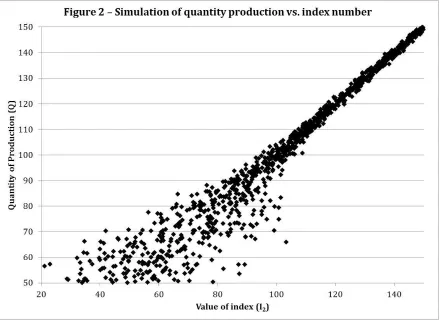
regression-approach from Vedenov and Barnett. Notice also how the two graphs have opposite variance structures. The points are tightly concentrated around the best fit line for low values of production and loosely dispersed around the line for high values of production in Figure 1. Again, this occurs by construction: it allows me to emphasize the role that model accuracy plays in effectiveness of an index derivative. All of these

(11)

[image:11.612.88.528.72.392.2]

A careful reader may also notice that the dispersion of points is generally smaller in Figure 2 than Figure 1. Again, this occurs by construction: I pick parameter values in the volatility structure to ensure that the explanatory power for index #2 is stronger than index #1. To quantify this idea, I calculate the sum of squared residuals (SSR), which is a measure of statistical explanatory power defined in Equation (13).

(13) 𝑆𝑆𝑅 = [∑(𝑄 − 𝐼)2]12

Smaller values of SSR are associated with stronger statistical power. Vedenov and Barnett use a different measure of explanatory power, the coefficient of determination (R2_).

I do not work with R2_{because it is not necessarily bounded between zero and one for data}

(12)

I report the explanatory power for each index in Table 1. The results show that index #1 has less explanatory power than index #2. Based on my interpretation of Vedenov and Barnett, this implies that index #2 is better than #1 in terms of statistical explanatory power.

Table 1 – Comparison of explanatory power

Index #1 Index #2 SSR 366.09 235.51

To conclude my simulation experiment, I propose a derivatives for each index and compare the benefit for each within my framework. Since the two indices both have a linear relationship to quantity of production, it is appropriate to use a vanilla put option to hedge risk of low production. I calculate the net payoff for the put option according to Equation (14). Notice that the payoff for each derivative is based on the index, not quantity of production. This occurs because the index derivative provides an indirect hedge, a derivative on the index number and not production itself.

(14) N(I|Θ) = q[(K-I)+_{- O(K)]}

Equation (14) is the standard expression for payoff of a put option. There are two parameters: strike, K, and quantity or coverage, q. For simplicity, I assume that each option provides full coverage (100% coverage), as in Vedenov and Barnett and the insurance literature (2001, pg. 394). Full coverage implies that the strike for the put option equals average level of production (K=Q̅) and quantity equals one (q=1). Although this is useful as an illustration, it is not necessarily the optimal specification for the shape parameters; I leave the optimization for subsequent research because my goal here is to establish existence of a special case. Based on a put option with full coverage, I calculate the distribution of profit with each type of derivative according to Equation (15) and (16).

(15) Π₁ = Π₀+ N(I₁|q = 1, K = 100)

(13)

I calculate the premium for each derivative as expected payoff, which implies that the expected net payoff for the derivative is equal to zero, E(N(I|Θ))=0. Furthermore, this assumption implies that the expected profit with either derivative is equal to the profit without the derivative. However, the higher moments of the payoff function are non-zero, which leads me to use numerical analysis to investigate the entire distribution of profit with or without each type of index derivative.

Figures 3 and 4 show how each derivative affects the distribution of profit. The figures show a scatterplot of simulated profits. Each data point denotes the level of profit with and without the derivative based on a simulated value for the quantity and index number. The graphs are similar to a Q-Q plot (quantile-quantile plot) from statistics: if the two distributions are the same, then all points will fall on the 45° line through the origin (Y=X), which is denoted by a red dotted line. However, the observed data do not generally lie on the red dotted line for two main reasons: first, the premium for the derivative shifts profits downwards in the good times; second, the payoff from the derivative shifts the profit upwards in bad times.

Figure 3 compares the distribution of profitability for the derivative on index #1 versus no derivative. The dotted line denotes where the data points would fall if the producer bought zero units of the derivative. Points above the dotted line represent outcomes where the producer has larger profit with the derivative than without, points below represent outcomes where the producer has smaller profit with the derivative.

I use two red circles in Figure 3 to identify two stylized facts about the effect of the derivative. The circle denoted as Region A shows where the index derivative is working well. The profit without the derivative is low (between 60 and 90, along the horizontal axis), but the profit with the derivative is concentrated around a much higher value

(14)

(15)

[image:15.612.86.531.386.709.2]

Figure 4 compares the distribution of profitability for the derivative on index #2 versus no derivative. Region C shows the region where the derivative is supposed to work, but the large dispersion of points shows that the derivative is not reliable. The dispersion in Region C occurs because index #2 is inaccurate for low levels of profit. There are some points in Region C where the derivative offsets losses and causes high payoffs but there are other points where profit is low both with and without the derivative. Region C shows that false negative errors occur often with index #2, which provides evidence that the

derivative is not working well from a risk management perspective. Furthermore, notice

that there is no ‘Region D’ in Figure 4 corresponding to Region B in Figure 3. There is no need for Region D because the index #2 is highly accurate for high values of production: there is low probability of false positives.

(16)

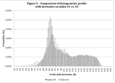
By my construction of the simulation experiment, profit with zero derivatives has a uniform between 50 and 150, Π₀~U(50,150). Both distributions in Figure 5 have much less weight in the ‘left tail’ than a uniform distribution, which implies that both derivatives can effectively hedge low profits. However, the distribution with index #1 has a smaller left tail than the distribution with index #2 and this suggests that index #1 is better than #2. Since risk management is generally concerned with the size and frequency of losses, this sort of graphical and heuristic-based comparison of the distributions can provide further insight into the relative efficiency of each index derivative based for the interested reader.

To analyze the results further within my modelling framework, I report several statistics for each distribution in Table 2. The results show that mean (average) profit is the same in each case, which is as expected because the derivative premium is calculated as expected payoff. Table 2 also shows that the standard deviation is lower with either

[image:16.612.77.522.430.559.2]

derivative than without, which suggests either derivative would benefit a risk-averse agent. However, the standard deviation of profits is even lower with index #1 than #2, which suggests that index derivative #1 would be preferred to #2 according to the mean-variance utility function.

Table 2 – Comparison of distribution of profit

No derivative Index #1 Index #2 Mean 101.11 101.11 101.11 Standard Deviation 28.89 16.64 17.68

Skewness -0.05 0.60 0.29 5% Quantile 66.74 81.61 75.51

(17)

Table 2 also presents the 5% Quantile for each distribution. The 5% Quantile is the value for which the following statement holds: with 95% probability, the producer will have profit greater than this value. The 5% Quantile is a useful measure of the left tail of the distribution and is based on the Value at Risk measure. The 5% Quantile for index #1 is higher than index #2, which suggests again that index #1 provides a better risk

management tool than index #2. All together, the results in Table 2 suggest index #1 is superior to index #2.

Discussion

In this paper I present a modelling framework for the design of financial derivatives. The model specifies that quantity of production is driven by a risk factor, or index number, and allows the producer to buy a derivative on the index number. The model assesses the benefit of the derivative in terms of the change in the distribution of profits. Although my model allows for a general statistical relationship between the quantity of production and the index number, I focus on a special case where the index is defined as the predicted value for quantity because this is related to an influential approach to creating new index numbers in agricultural risk management (Vedenov and Barnett, 2004).

I use my modelling framework to conduct a simulation experiment where I create two index numbers. Both have a linear relationship to quantity of production and a noise term with non-constant variance. The error for index #1 has low variance for low profit, which means it is accurate at predicting losses. The error for index #2 has high variance for low profit, which means it is inaccurate for predicting losses. I use the terminology of false positive and false negative errors to argue that index #1 is better than index #2 from a risk management perspective.

(18)

power. A possible reason for this result is that statistical power is measured over all values of quantity, whereas it may be sufficient for the index to have strong explanatory power only for low values of quantity to provide an effective hedge. Although my results are limited to particular parameter values, my results establish the existence of a special case that validates the following statement: strong explanatory power does not necessarily imply strong risk management power.

My research method uses a theoretical probability distribution to conduct numerical simulation for a complicated, stochastic economic model. Simulation with large samples approximates a continuous, algebraic solution, but it raises an important question: is my research theoretical economics? Uskali Mäki suggests that “only theoretical modeling [sic]

qualifies as proper modeling” in economics, which includes algebraic mathematics and excludes computer simulation or laboratory experimentation (Mäki, 2013, pg. 88).

Therefore, my research is not theoretical according Mäki. Neither is my research empirical, in the sense of using real-world data. Instead, my research resembles a ‘simple model’ in computational social science. Dirk Helbing characterizes simple models as those that use a

“minimum number of variables needed to reproduce a certain effect, phenomenon, or

(19)

References

Bell, P. (2014). Optimal use of put options in a stock portfolio. Unpublished manuscript. Available from http://mpra.ub.uni-muenchen.de/54871/

Heimfart, L.E., & Musshoff, O. (2011). Weather index-based insurances for farmers in the North China Plain: An analysis of risk reduction potential and basis risk. Agricultural Finance Review, 71(2), 218-239.

Helbing, D. (2013). Pluralistic Modeling of Complex Systems. In U. Gӓhde, S. Hartmann, & J. H. Wolf (Eds.), Models, Simulations, and the Reduction of Complexity (53-80). Berlin, Germany: Walter de Gruyter GmbH.

Turvey, C. G. (2001). Weather Derivatives for Specific Event Risk in Agriculture. Review of Agricultural Economics, 23(2), 333–351.

Mäki, U. (2013). Contested Modeling: The Case of Economics. In U. Gӓhde, S. Hartmann, & J. H. Wolf (Eds.), Models, Simulations, and the Reduction of Complexity (87-106). Berlin, Germany: Walter de Gruyter GmbH.

(20)

Appendix A

Matlab code to replicate all results

%% Simulation File by Peter Bell, July 2014 %

%% Section 1: Simulate data for production and risk factor

clear all

s=RandStream('mt19937ar','Seed',125); RandStream.setGlobalStream(s);

sampSize=1000; yieldSim=50+100*rand(sampSize,1);

sigmaOne=zeros(sampSize,1); sigmaTwo=zeros(sampSize,1); noiseOne=zeros(sampSize,1); noiseTwo=zeros(sampSize,1); indexOne=zeros(sampSize,1); indexTwo=zeros(sampSize,1); bestFit=zeros(sampSize,1);

aNo = 1; kNo = 15; bNo = 0.1; vNo = 0.5; qNo = 0.5; mNo =80;

for iDraw = 1:sampSize

sigmaOne(iDraw) = aNo + (kNo - aNo)/(1+qNo*...

exp(-bNo*(yieldSim(iDraw)- mNo)))^(1/vNo); sigmaTwo(iDraw) = kNo - (kNo - aNo)/(1+qNo*...

exp(-bNo*(yieldSim(iDraw)- mNo)))^(1/vNo);

noiseOne(iDraw) = randn(1,1)*sigmaOne(iDraw); noiseTwo(iDraw) = randn(1,1)*sigmaTwo(iDraw); bestFit(iDraw) = yieldSim(iDraw);

indexOne(iDraw) = bestFit(iDraw)+noiseOne(iDraw); indexTwo(iDraw) = bestFit(iDraw)+noiseTwo(iDraw);

end

%% Section 2: Backtest put option

strike = 100; % Set strike at average production, Q ~ U(50,150)

quantOpt = 1; % Buy one unit of put options

payoffOne = max( (strike.*ones(sampSize,1)-indexOne), 0); payoffTwo = max( (strike.*ones(sampSize,1)-indexTwo), 0);

premOne=mean(payoffOne); premTwo=mean(payoffTwo);

backtestOne = yieldSim + quantOpt*( payoffOne - premOne.*ones(sampSize,1)); backtestTwo = yieldSim + quantOpt*( payoffTwo - premTwo.*ones(sampSize,1));

%% Section 3: Save data for graphics

% Figures 1 and 2: Shows yield versus index

figureOne = [ yieldSim, indexOne]; figureTwo = [ yieldSim, indexTwo];

(21)

% Figures 3 and 4: Shows profit with derivative versus without

figureThree = [ yieldSim, backtestOne]; figureFour = [ yieldSim, backtestTwo];

save('FigureThree-Profits.txt','figureThree', '-ascii', '-tabs') save('FigureFour-Profits.txt','figureFour', '-ascii', '-tabs')

% Figures 5 and 6: Marginal distribution of profit with index derivative

binLoc = 50:1:150;

[histFreqOne,histLocOne] = hist(backtestOne,binLoc); % [histFreqOne,histLocOne]

[histFreqTwo,histLocTwo]= hist(backtestTwo,binLoc); histOne = [histFreqOne', histLocOne'];

histTwo = [histFreqTwo', histLocTwo'];

save('FigureFive-HistOne.txt','histOne', '-ascii', '-tabs') save('FigureFive-HistTwo.txt','histTwo', '-ascii', '-tabs')

%% Section 4: Calculate statistics from distribution

for i =1:sampSize

SSROne(i) = (yieldSim(i)-indexOne(i))^2; SSRTwo(i) = (yieldSim(i)-indexTwo(i))^2;

end

tableOne = [sum(SSROne)^0.5, sum(SSRTwo)^0.5];

save('TableOne-SSR.txt','tableOne', '-ascii', '-tabs')

yieldSim = sort(yieldSim);

backtestOne = sort(backtestOne); backtestTwo = sort(backtestTwo);

% Note: sorting breaks relationship across variables

tableTwo = [ mean(yieldSim), mean(backtestOne), mean(backtestTwo);...

std(yieldSim), std(backtestOne), std(backtestTwo);...

skewness(yieldSim), skewness(backtestOne), skewness(backtestTwo);...

yieldSim(50), backtestOne(50), backtestTwo(50) ]; save('TableTwo-RiskStats.txt','tableTwo', '-ascii', '-tabs')