Munich Personal RePEc Archive
Sign-based specification tests for
martingale difference with conditional
heteroscedasity
Chen, Min and Zhu, Ke
Chinese Academy of Sciences and Capital University of Economics
and Business, Chinese Academy of Sciences
1 June 2014
Online at
https://mpra.ub.uni-muenchen.de/56347/
Sign-based specification tests for martingale difference with
conditional heteroscedasity
BYMINCHEN
Chinese Academy of Sciences and Capital University of Economics and Business
ANDKEZHU
Chinese Academy of Sciences
ABSTRACT
This article proposes Cram´er-von Mises (CM) and Kolmogrove-Smirnov (KS) test statistics 10
based on the signs of a time series to test the null hypothesis that the series is a martingale
difference sequence (MDS) with conditional heteroscedasity. Both of test statistics allowing for
heavy-tailedness, non-stationarity, and nonlinear serial dependence of unknown forms, are
easy-to-implement. Unlike the sign-based variance-ratio test in Wright (2000), our sign-based CM
and KS tests have no need to select the lag. Unlike other often used specification tests for MDS, 15
our sign-based CM and KS tests are robust and have exact distributions which can be simulated
easily. Simulation studies and applications further demonstrate the importance of our sign-based
CM and KS tests.
Some key words: Conditional heteroscedasity; Cram´er-von Mises test; Kolmogrove-Smirnov test; Martingale
differ-ence; Robustness. 20
1. INTRODUCTION
One of the most important questions in applied econometrics and empirical finance is the issue
of whether a time series such as the stock-market and exchange-rate returns forms a martingale
see, e.g., Timmermann and Granger (2004) and Lim and Brooks (2011). Once a time series is a
25
MDS, it is unpredictable; otherwise, there has a practical demand to fit its conditional mean by
some useful models. Thus, testing for MDS is meaningful and has been popular in the literature;
see, e.g., Durlauf (1991) and Deo (2000) for earlier works and Escanciano (2007) and the
refer-ences therein for more recent ones. Moreover, for most of economics and financial datayt, if it
is a MDS, it often admits a conditional heteroscedastic form as follows:
30
yt=εtσt, (1.1)
whereE(εt|Ft−1) = 0,σt∈ Ft−1 is positive, andFt is aσ-field generated by{yt, yt−1,· · · }.
This feature ofythas been more or less accepted in application after the seminal work of Engle
(1982) and Bollerslev (1986). Many existing models, such as the GARCH model and its vast
variants (see, e.g., Fan and Yao (2003) or Tsay (2005) for an overview), the stochastic volatility
35
model in Shephard (1996), the conditional piecewise constant volatility model in Chan et al.
(2014) to name but a few, are nested by model (1.1). Thus, it is desirable to detect the following
null hypothesis:
H0:ytadmits the form as in(1.1).
Needless to say, the Cram´er-von Mises (CM) test based on sample autocorrelations of{yt}in
40
Deo (2000) and the CM and Kolmogrove-Smirnov (KS) tests based on some marked processes in
Escanciano (2007) are both valid for this purpose; see also Hong (1996, 1999), Shao (2011a, b),
Zhu and Li (2014) and references therein for testing the null hypothesis thatytis a white noise.
However, whenytis heavy-tailed with an infinite variance (see, e.g., Davis and Mikosch (1998),
Rachev (2003) and Zhu and Ling (2014) for some empirical examples in this context), none of
45
existing tests except the sign-based variance-ratio (VR) test in Wright (2000) is feasible. In this
paper, we propose the sign-based CM and KS tests to detect H0. Both of our sign-based CM
and KS tests allowing for heavy-tailedness, non-stationarity, and nonlinear serial dependence of
unknown forms, are easy-to-implement. Unlike the sign-based VR test in Wright (2000), our
sign-based CM and KS tests have no need to select the lag. Unlike other aforementioned tests
50
for MDS, our sign-based CM and KS tests are robust and have exact distributions which can be
simulated easily. Simulation studies and applications further demonstrate the importance of our
This paper is organized as follows. Section 2 gives our test statistics and their exact
distribu-tions. Simulation results are reported in Section 3. Applications are given in Section 4. Conclud- 55
ing remarks are offered in Section 5.
2. TEST STATISTIC AND EXACT DISTRIBUTION
The use of sign-based tests in regression and time series models so far has attracted
consider-able interest; see, e.g., Koenker and Bassett (1982), Wright (2000), Hallin et al. (2008), Coudin
and Dufour (2009), Chen and Zhu (2014), Zhu and Ling (2014), and many others. In this section, 60
based on the signs of{yt}, we propose the CM and KS tests to detectH0.
Denote by sgn(yt) := 2I(yt>0)−1 the sign of yt, where I(·) is the indicator function. Let γ(j) =cov(st, st+j) with st=sgn(yt). Then, the spectral density function and spectral distribution function ofst, respectively, are
f(ω) = 1 2π
∞
X
j=−∞
γ(j)e−ijω forω∈[−π, π]
andF(λ) =Rλ
0 f(ω)dωforλ∈[0, π]. Following Shao (2011a), the sample spectral distribution
function ofstis
Fn(λ) =
n−1
X
j=0
ˆ
γ(j)ψj(λ),
whereγˆ(j) =n−1Pn
t=1+|j|(st−s¯)(st−|j|−s¯) is the sample autocovariance function ofst at lagj,¯s=n−1Pn
t=1stis the sample mean ofst, and
ψj(λ) = ½
sin(jλ)/jπ ifj6= 0 λ/2π ifj= 0 .
Moreover, to validate our test statistics, we need the following assumption as in Wright (2000):
Assumption2.1. I(εt>0)is an i.i.d. binomial random variable that is1with probability1/2 and0otherwise.
Assumption 2.1 holds whenεtis an i.i.d. random variable with a median zero and a continuous 65
pdf at zero, and hence it allows for the heavy-tailedεtas in Berkes and Horv´ath (2004), Linton et
al. (2010), and Chen and Zhu (2014). In addition, since the i.i.d. assumption onεtis not necessary
from Assumption 2.1, εt could also be t-distributed with time-varying degrees of freedom as
Based on Assumption 2.1, it is straightforward to see that underH0,{st}is an i.i.d. binomial
70
variable that is1with probability1/2and−1otherwise. This implies thatF(λ) =γ(0)ψ0(λ)
underH0, and the sample spectral distributionFn(λ) becomesˆγ(0)ψ0(λ) in this case. Thus, it
is reasonable to consider the following sign-based CM and KS test statistics to detectH0, where
CMn= Z π
0
Sn2(λ)dλ, KSn= max
λ∈[0,π]S
2
n(λ), (2.1)
and the process
Sn(λ) =√n{Fn(λ)−γˆ(0)ψ0(λ)}=:
n−1
X
j=1
√
nγˆ(j)ψj(λ)
measures the distance betweenFn(λ)andˆγ(0)ψ0(λ). Clearly, CMnor KSntakes into account
75
of the autocorrelations ofstat all lags, and a large value of CMnor KSnis in favor of rejecting
H0. Next, we give the exact null distributions of CMnand KSnin the following theorem:
THEOREM2.1. Suppose that Assumption2.1holds. UnderH0, CMnand KSnhave the same
distribution as
Z π
0
[Sn∗(λ)]2dλ and max
λ∈[0,π][S
∗
n(λ)]2,
respectively, where
Sn∗(λ) = √1
n
n−1
X
j=1
n X
t=1+j
(s∗t −s¯∗)(s∗t−j−s¯∗)ψj(λ),
{s∗
t}nt=1is an i.i.d. sequence, each element of which is1with probability1/2and−1otherwise,
ands¯∗=n−1Pn
t=1s∗t.
Remark2.1. The CM test based on{yt}itself has been studied by Shao (2011a), and our CM
80
test based on {st}can be viewed as a robust version of his test. Compared to the CM test in Shao (2011a) and the CM and KS tests in Escanciano (2007), our sign-based CM and KS tests
only take into account of the signs of{yt}, and hence they may not be consistent. But, our sign-based tests also have three potential advantages: first, neither finite second moment condition
nor stationarity ofytis needed; second, no bootstrap procedure is required to obtain the critical
85
values; third, the technical difficulty in proving the tightness for the test statistic is circumvented.
Remark2.2. From Theorem 2.1, we know that our sign-based CM and KS tests allow for
also the case for the Wright’s (2000) sign-based variance-ratio (VR) test defined by
VRn(k) = " Pn
t=k+1(st+st−1+· · ·+st−k+1)2 kPn
t=1s2t −
1
#
×
·
2(2k−1)(k−1) 3kn
¸−1/2
,
wherekis the lag parameter. Numerical studies in Wright (2000) showed that the performance
of VRn(k)is sensitive tok, but how to choose the optimal kis hard in theory. Our sign-based CM and KS tests do not face this dilemma, since they are free of user-chosen parameter.
Remark2.3. In application, one may consider the following null hypothesisH0′ instead ofH0: 90
H0′ :yt=µ+εtσt,
whereµis an unknown parameter. To detectH0′, it may be natural to first estimateµby med(yt) (i.e., the sample median of{yt}), and then apply both CMnand KSnto the adjusted series{y˜t}, wherey˜t=yt−med(yt). However, we can see thatsgn(˜yt)6=sgn(εt)due to the estimation of
µ. Thus, this aforementioned method is not valid, and the portmanteau test based on the bootstrap 95
method in Zhu and Ling (2014) should be used to detectH0′.
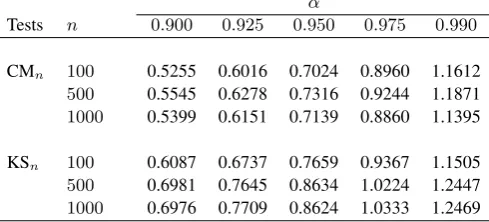
Based on 20,000 repetitions, Table 1 reports the100(1−α)% percentiles of the exact null distributions of CMnand KSnfor some choices ofnandα. Then, we rejectH0at the significance
[image:6.595.183.428.451.562.2]levelα, when the value of CMnor KSnis larger than the corresponding percentile.
Table 1.100(1−α)%percentiles of the exact null distributions of CMnand KSn. α
Tests n 0.900 0.925 0.950 0.975 0.990
CMn 100 0.5255 0.6016 0.7024 0.8960 1.1612
500 0.5545 0.6278 0.7316 0.9244 1.1871
1000 0.5399 0.6151 0.7139 0.8860 1.1395
KSn 100 0.6087 0.6737 0.7659 0.9367 1.1505
500 0.6981 0.7645 0.8634 1.0224 1.2447
1000 0.6976 0.7709 0.8624 1.0333 1.2469
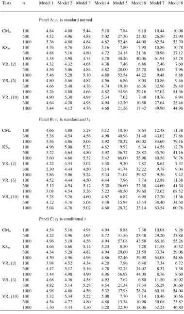
3. SIMULATIONS 100
There are an enormous number of ways of testingH0; see, e.g., Chen and Deo (2006), Shao
(2011a), and refrences therein. The simulation studies we conduct in this section do not attempt
to compare all possible tests but only the based VR test in Wright (2000), because the
sign-based VR test enjoys the same simplicity and robustness as ours. The goal is limited. But if our
in some plausible models, then it follows that our new tests should be useful specification tests
for practitioners.
The models we use to examine the size and power performance of all sign-based tests are as
follows:
Model 1:yt=εtexp(ht/2), ht= 0.95ht−1+ξt, ξt∼i.i.d.N(0,0.1),
110
Model 2:yt=εt p
ht, ht= 0.1 + [0.2 + 0.1I(εt−1 <0)]yt2−1+ 0.8ht−1,
Model 3:yt=εt p
ht, ht= 0.1 + 0.1[1−0.4sgn(εt−1) + 0.04]y2t−1+ 0.9ht−1,
Model 4:yt=εt p
ht, ht= 0.1 + 0.147yt2−1+ 0.926ht−1,
Model 5:yt= 0.1yt−1+νt, whereνtis defined asytin model 1, Model 6:yt= 0.1yt−1+νt, whereνtis defined asytin model 2,
115
Model 7:yt= 0.2yt−2+νt, whereνtis defined asytin model 3, Model 8:yt= 0.2yt−2+νt, whereνtis defined asytin model 4.
Clearly, models 1-4 which admit the specification of MDS with conditional heteroscedasticity are
used for the size simulation study, and the remaining models are used for the power simulation
study. Specifically, model (1) is the stochastic volatility model of conditional heteroscedasticity
120
used in Wright (2000); models (2)-(3) used in Zhu and Ling (2014) are GJR model and non-linear
GARCH model withEyt2=∞, respectively; model (4) is a non-stationary GARCH model used in Francq and Zako¨ıan (2012) for fitting KVA series; and models (5)-(8) deviate from models
(1)-(4) by an AR model, respectively. In each of these eight models,εtis i.i.d. standard normal,
standardizedt3 with variance one, ortηt, where the degree of freedomηt is dynamically
gen-125
erated fromηt= 27.9/(1 + exp(−λt)) + 2.1andλt=−1.07−0.38εt−1−0.08ε2t−1. The last
choice fortηt is taken from Hansen (1994), who used the logistic transformation to bound the
degrees of freedomηtbetween 2.1 and 30.
As Wright (2000), we generate 5000 replications of sample sizen= 100,500and1000from each aforementioned model. For each replication, we use the tests CMn, KSn, and VRn(k)for
130
k= 2,5,10to detectH0. Table 2 reports the size and power of all tests based on the significance
levelα= 0.05, where the critical values of CMnand KSnare taken from Table 1, and the critical values of VRn(k)are taken from Table 1 in Wright (2000). From Table 2, it is clear that the sizes of these tests are close to their nominal ones, and the power of them is generally as expected.
First, all the powers become large asnincreases. Second, each test has a larger power when the
135
Table 2.Empirical sizes and power (×100) for all sign-based tests.
Tests n Model 1 Model 2 Model 3 Model 4 Model 5 Model 6 Model 7 Model 8
Panel A:εtis standard normal
CMn 100 4.84 4.80 5.44 5.10 7.84 8.10 10.44 10.08
500 4.52 4.96 4.88 5.02 27.30 23.02 26.50 22.90
1000 5.36 4.80 4.84 4.62 52.48 44.00 62.54 53.20
KSn 100 4.76 4.76 5.06 5.16 7.80 7.90 10.86 10.78
500 4.88 5.16 4.80 4.72 24.18 21.36 30.96 27.12
1000 5.38 4.98 4.74 4.70 48.26 40.06 61.94 53.78 VRn(2) 100 4.32 4.32 4.68 4.38 7.46 6.86 7.46 7.60
500 4.56 5.06 4.84 4.82 28.00 23.70 8.00 7.96
1000 5.46 5.28 5.10 4.80 52.54 44.22 9.48 8.88
VRn(5) 100 4.80 4.66 4.84 4.56 6.86 8.04 10.86 9.46
500 4.66 5.48 4.76 4.74 19.10 16.36 32.96 29.40
1000 5.26 4.88 4.66 4.82 34.96 29.16 57.02 51.36 VRn(10) 100 4.90 5.30 4.98 5.34 7.02 7.48 10.76 8.94
500 4.64 4.28 4.98 4.94 12.20 10.58 27.64 25.46
1000 5.44 4.12 4.76 4.68 21.26 17.42 49.90 44.96
Panel B:εtis standardizedt3
CMn 100 4.66 4.88 5.28 5.12 10.10 8.64 12.48 11.38
500 5.38 4.54 4.56 4.98 40.96 31.40 43.02 37.86
1000 5.56 4.86 5.06 4.92 70.32 60.02 84.60 79.16
KSn 100 4.96 5.08 5.22 4.82 9.92 8.34 14.58 12.76
500 5.22 4.64 4.80 4.92 36.72 28.82 45.70 41.16
1000 5.60 4.66 5.32 5.42 66.00 55.98 80.56 76.76 VRn(2) 100 4.22 4.34 5.02 4.30 9.20 7.82 8.64 7.32
500 5.30 4.44 4.50 5.14 41.74 32.22 9.78 9.04
1000 5.86 5.06 5.24 5.34 71.04 59.82 9.36 9.42
VRn(5) 100 4.52 4.44 4.50 4.44 7.96 7.74 12.88 11.38
500 5.12 4.54 5.12 5.30 26.60 22.38 44.60 41.34
1000 5.08 4.54 5.26 5.22 48.50 39.60 72.02 68.52 VRn(10) 100 5.28 5.26 4.60 4.62 6.82 6.90 12.20 11.36
500 4.72 4.76 5.04 4.48 15.94 13.54 38.40 34.50
1000 5.04 4.76 5.02 4.60 28.72 23.14 63.54 60.76
Panel C:εtis conditionalt
CMn 100 4.54 5.16 4.98 4.94 8.88 7.38 10.08 9.26
500 4.22 4.96 4.94 4.72 31.56 23.48 29.20 23.88
1000 4.96 5.18 4.56 4.94 57.08 43.58 65.16 55.26
KSn 100 4.66 4.66 5.14 5.24 8.50 7.28 11.58 10.52
500 4.34 5.28 4.82 4.94 29.60 21.50 33.34 29.06
1000 4.50 4.96 4.96 4.86 52.46 39.90 64.08 54.86 VRn(2) 100 3.98 4.52 4.34 4.20 7.96 6.48 7.34 6.72
500 4.42 5.12 5.16 4.78 32.24 24.02 8.32 7.38
1000 5.44 4.98 4.90 4.96 56.98 44.00 8.76 8.60
VRn(5) 100 4.68 4.36 4.58 4.92 7.62 6.80 11.20 10.02
500 4.82 5.14 5.28 4.54 21.34 17.34 35.28 30.60
1000 4.98 4.86 4.56 5.32 37.98 28.24 60.18 54.04 VRn(10) 100 5.32 5.34 5.22 5.08 7.70 7.14 10.46 10.56
500 4.54 4.72 4.80 4.88 13.34 10.98 30.08 25.82
power performance of VRn(k)becomes worse askincreases, while whenytexhibits the second order autocorrelation as in models 7-8, VRn(2)has a very low power since it can only detect the first order autocorrelation, and the power of VRn(5)is higher than that of VRn(10). Fourth, CMn and KSn, taking into account of the autocorrelations at all lags, always have a competitive power
140
performance with regard to the best performing VRn(k). Overall, simulation studies indicate that both CMnand KSnhave a good power performance with no risk of lag-selection as in VRn(k) or size distortions.
4. APPLICATION
In this section, we apply the sign-based tests to several exchange rate series. The data sets
we studied are the four daily currencies against the U.S. dollar, the Argentine Peso (USD/ARS),
Chinese Yuan (USD/CNY), Colombian Peso (USD/COP), and Malaysian Ringgit (USD/MYR),
over the period from November 14, 2009 to August 10, 2012. They are the currencies from the
developing countries, two from Latin America and two from Asia. Each series has a total of
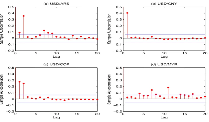
1001 observations. Denote the log-return (×100) of each series by{yt}nt=1 withn= 1000. A
simple visual inspection of the sample autocorrelation plots of{y2
t}nt=1 in Figure 1 implies that
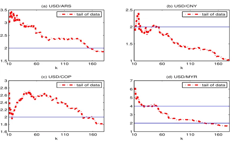
all return series are highly correlated with possible ARCH effect. Moreover, Figure 2 plots the
Hill’s estimators{Hy(k)}180k=10for each return series, where
Hy(k) = "
1 k
k X
i=1
log y(n−i) y(n−k)
#−1
with{y(t)}nt=1being the ascending order statistics of{yt}nt=1. From Figure 2, it is reasonable to
145
conclude that the tail indexes of USD/ARS, USD/COP, and USD/MYR return series are less than
4, and the tail index of USD/CNY return series is even less than 2. Thus, it is reasonable to use all
sign-based tests to detect whether each return series is a MDS with conditional heteroscedasity.
Table 3 reports all of the results for each sign-based test. From this table, we find that (i)
the tests CMn, KSn, and VRn(5)imply that USD/ARS return series is not a MDS, while this
150
can not be detected by others; (ii) all tests indicate that USD/CNY return series is a MDS; (iii)
the tests CMn, KSn, and VRn(2)have a very strong evidence to reject the MDS hypothesis for USD/COP return series, but this can not be detected by VRn(5)or VRn(10); and (iv) only KSn can reject the MDS hypothesis for USD/MYR return series. Overall, our sign-based tests CMn
and KSngive more consistent and much stronger rejections, while the results using the VRn(k)
155
0 5 10 15 20 −0.2 −0.1 0 0.1 0.2 0.3 0.4 0.5 Lag Sample Autocorrelation (a) USD/ARS
0 5 10 15 20
−0.2 −0.1 0 0.1 0.2 0.3 0.4 0.5 Lag Sample Autocorrelation (b) USD/CNY
0 5 10 15 20
−0.2 −0.1 0 0.1 0.2 0.3 0.4 0.5 Lag Sample Autocorrelation (c) USD/COP
0 5 10 15 20
[image:10.595.98.507.103.342.2]−0.2 −0.1 0 0.1 0.2 0.3 0.4 0.5 Lag Sample Autocorrelation (d) USD/MYR
Fig. 1. Sample autocorrelation functions of{y2
t}for four different exchange rates.
results. It means that people in the exchange market can not get profit via predicting the value
of USD/CNY. The reason is probably because CNY is not a freely convertible currency, and
the USD/CNY is a managed floating exchange rate released by the People’s Bank of China. For
other aforementioned exchange rates, they do not have such a mechanism like USD/CNY, and 160
people in these exchange markets can possibly conduct prediction by their own strategy.
Table 3.The values of all sign-based tests.
Return series
Tests USD/ARS USD/CNY USD/COP USD/MYR
CMn 0.7617∗ 0.3794 1.2382*** 0.5413
KSn 1.1132** 0.3974 1.8229*** 0.9610∗
VRn(2) -0.7589 1.8341 2.5931*** 1.5179
VRn(5) -2.0005∗ 0.7939 0.5167 0.0318
VRn(10) -0.9029 1.6521 1.2288 0.2323
a The test statistics have one, two, or three stars if significant at the level 5%,
[image:10.595.163.451.501.665.2]10 60 110 160 1.5
2 2.5 3 3.5
k (a) USD/ARS
10 60 110 160
1 1.5 2 2.5
k (b) USD/CNY
10 60 110 160
1.6 1.8 2 2.2 2.4 2.6 2.8 3
k (c) USD/COP
10 60 110 160
1 2 3 4 5 6 7
k (d) USD/MYR tail of data
tail of data tail of data
[image:11.595.96.486.100.347.2]tail of data
Fig. 2. Hill’s estimators{Hy(k)}
180
k=10for four different exchange rates.
5. CONCLUDING REMARKS
In this paper, we propose the sign-based CM and KS tests to detect the null hypothesis that
the series is a MDS with conditional heteroscedasity. By only checking the autocorrelations of
the signs, our new tests may not be consistent. However, as a compensation, our new tests allow
165
for heavy-tailedness, non-stationarity, and nonlinear serial dependence of unknown forms.
Par-ticularly, they have the exact distributions, and hence no time-consuming bootstrap procedure is
needed to obtain the critical values, and the size-distortion is not a problem any more. Generally,
this is not the case for existing specification tests except the sign-based VR test in Wright (2000).
Compared to Wright’s (2000) test, our sign-based tests do not need to choose the lag parameter.
170
This is indeed important, because simulation studies show that the power of sign-based VR test
depends heavily on the choice of the lag, but our sign-based tests can always give a
competi-tive power performance with regard to the best performing sign-based VR tests. Moreover, the
empirical application shows that our sign-based CM and KS tests can give more consistent and
much stronger rejections than the sign-based VR tests. Thus, in view of these, it is reasonable to
175
ACKNOWLEDGEMENT
This work is supported by the National Natural Science Foundation of China (No.10990012,
11021161, 11371354, and 11201459).
REFERENCES 180
[1] BERKES, I. and HORVATH, L. (2004). The effciency of the estimators of the parameters in GARCH processes.´
Annals of Statistics32, 633–655.
[2] BOLLERSLEV, T. (1986). Generalized autoregressive conditional heteroskedasticity. Journal of Econometrics
31, 307–327.
[3] CHAN, K.-S., LI, D., LING, S. and TONG, H. (2014). On conditionally heteroscedastic AR models with 185
thresholds.Statistica Sinica24, 625–652.
[4] CHEN, M. and ZHU, K. (2014). Sign-based portmanteau test for ARCH-type models with heavy-tailed
innova-tions. Forthcoming inJournal of Econometrics.
[5] CHEN, W. and DEO, R.S. (2006). The variance ratio statistic at large horizons. Econometric Theory22,
206–234. 190
[6] COUDIN, E. and DUFOUR, J.-M. (2009). Finite-sample distribution-free inference in linear median regressions
under heteroscedasticity and non-linear dependence of unknown form.Econometrics Journal12, S19–S49.
[7] DAVIS, R.A. and MIKOSCH, T. (1998). The sample autocorrelations of heavy-tailed processes with applications
to ARCH.Annals of Statistics26, 2049–2080.
[8] DEO, R.S. (2000). Spectral tests of the martingale hypothesis under conditional heteroskedasticity.Journal of 195
Econometrics99, 291–315.
[9] DURLAUF, S.N. (1991). Spectral-based testing of the martingale hypothesis. Journal of Econometrics50,
355–376.
[10] ENGLE, R.F. (1982). Autoregressive conditional heteroskedasticity with estimates of variance of U.K. inflation.
Econometrica50, 987–1008. 200
[11] ESCANCIANO, J.C. (2007). Model checks using residual marked emprirical processes. Statistica Sinica17,
115–138.
[12] FAN, J. and YAO, Q. (2003). Nonlinear time series: Nonparametric and parametric methods. Springer, New
York.
[13] FRANCQ, C. and ZAKO¨IAN, J.M. (2012). Strict stationarity testing and estimation of explosive and stationary 205
generalized autoregressive conditional heteroscedasticity models. Econometrica80, 821–861.
[14] HALLIN, M., VERMANDELE, C., and WERKER, B. (2008). Semiparametrically efficient inference based on
signs and ranks for median-restricted models.Journal of the Royal Statistical Society, Series B70, 389–412.
[15] HANSEN, B.E. (1994). Autoregressive conditional density estimation. International Econoinic Review35,
705–730. 210
[17] HONG, Y. (1999). Hypothesis testing in time series via the empirical characteristic function: A generalized
spectral density approach.Journal of the American Statistical Association94, 1201–1220.
[18] KOENKER, R. and BASSETT, G. (1982). Tests of linear hypotheses andL1 estimation. Econometrica50,
1577–1584.
215
[19] LIM, K.-P. and BROOKS, R. (2011). The evolution of stock market efficiency over time: a survey of the
empirical literature.Journal of Economic Surveys25, 69–108.
[20] LINTON, O., PAN, J. and WANG, H. (2010). Estimation for a non-stationary semi-strong GARCH(1,1) model with heavy-tailed errors.Econometric Theory26, 1–28.
[21] RACHEV, S.T. (2003). Handbook of Heavy Tailed Distributions in Finance. Elsevier/North-Holland.
220
[22] SHAO, X. (2011a). A bootstrap-assisted spectral test of white noise under unknown dependence. Journal of
Econometrics162, 213–224.
[23] SHAO, X. (2011b). Testing for white noise under unknown dependence and its applications to diagnostic
checking for time series models.Econometric Theory27, 312–343.
[24] SHEPHARD, N. (1996). Statistical aspects of ARCH and stochastic volatility. In D.R. Cox, D.V. Hinkley, &
225
O.E. Barndorff-Nielsen (eds.),Time Series Models in Econometrics, Finance and Other Fields. Chapman and
Hall.
[25] TIMMERMANN, A. and GRANGER, C.W.J. (2004). Efficient market hypothesis and forecasting.International
Journal of Forecasting20, 15–27.
[26] TSAY, R.S. (2005).Analysis of financial time series (2nd ed.). New York: John Wiley & Sons, Incorporated.
230
[27] WRIGHT, J.H. (2000). Alternative variance-ratio tests using ranks and signs.Journal of Business & Economic
Statistics18, 1-9.
[28] ZHU, K. and LI, W.K. (2014). A bootstrapped spectral test for adequacy in weak ARMA models. Working
paper. The university of Hong Kong.
[29] ZHU, K. and LING, S. (2014). Inference for ARMA models with unknown-form and heavy-tailed
G/ARCH-235