Munich Personal RePEc Archive
Physician quality and payment schemes:
A theoretical and empirical analysis
Calub, Renz Adrian
University of the Philippines School of Economics (UPSE)
June 2014
Online at
https://mpra.ub.uni-muenchen.de/92604/
1
Physician quality and payment schemes: A theoretical and
empirical analysis
*Renz Adrian T. Calub
**Abstract
Physicians are expected to provide the best health care to their patients; however, it cannot be discounted that their practice is driven primarily by incentives. In this paper, we construct a physician utility maximization model that links physician quality to compensation schemes. Results show that relative to fixed payment, fee-for-service and mixed payment yield higher quality. Multinomial treatment effects regression of vignette scores on payment schemes also support this hypothesis, indicating that physicians are still below the best level of quality and that incentives to improve are still present.
JEL Classification: I110, J440
Keywords: Physician, quality of healthcare, incentives, compensation schemes
1. Introduction
Equipped with the ability to produce health and prolong life, physicians bear a huge
responsibility in practicing their profession. With the patient’s life and future productivity in the
line, the health care profession is considered an esteemed field, operating within a set of guidelines and entry barriers to ensure quality [Arrow 1963]. However, benevolence may not always be expected from physicians. Like any economic agent, health providers have the capacity to alter his services given his financial incentives [Thorton & Eakin 1997]. Income is arguably an important factor in determining physician behavior, but the method of channeling such income to the physician should also be considered. For example, Barnum, Kutzin, and Saxenian [1995] argued that fixed payment tend to reduce services. Fee for service (FFS) tend to cause overprovision of services, while mixed payment appears to be a better alternative. Most studies have linked payment schemes with physician inputs such as work hours and services; however, using these inputs may not be sufficient to capture quality, an important dimension in the context of better health outcomes.
This paper attempts to construct a simple physician choice model that will allow us to compare quality of care across different payment schemes. The physician chooses his optimal effort level that will determine his quality given his income constraints which are then defined by each payment scheme. As an empirical support, the paper shall measure differences in scores derived from physician quality tests called the vignette across different payment schemes.
2. Payment schemes as incentive for quality
* This paper is a condensed version of the author’s Master’s thesis entitled “A theoretical and empirical analysis on
the relationship between payment schemes and physician quality”, May 2014.
** Master of Arts in Economics, University of the Philippines School of Economics (UPSE), Diliman, Quezon City
2
Payment schemes have been widely mentioned in the literature. Theoretical and empirical studies have identified payment schemes observed to increase or decrease motivation. In the health care sector, physicians can choose to work in any of the following payment arrangements [Barnum, Kutzin, & Saxenian 1995]:
1. Budgetary transfers – these are fixed, global budgets provided to the facility. Doctors are paid fixed remuneration depending on the total hospital budget.
2. Capitation – this is a typical scheme under insurance or health management offices (HMOs). Under this setup, physicians are paid a fixed amount per insured person. 3. Fee-for-service – this is a common practice in the industrialized countries where
providers charge according to the number of services provided.
4. Mixed payment scheme – this is a multi-dimensional payment scheme wherein providers can be paid in both fixed, budgetary transfers and fee-for-service. For
instance, a provider’s fixed cost can be paid through transfers while variable costs
may be reimbursed through fee-for-service payments.
2.1. Studies on payment scheme incentives: a review
Through their conceptual framework, Libby and Thurnston’s [2001] account on health management office (HMOs) hypothesized that entering into HMO/capitation arrangements generally decrease work hours. Physicians are motivated to enter such arrangement to reduce variability in working hours, to comply with group practice decisions, and to advocate managed care which is associated with lower cost of care due to early prevention and intervention. On the other hand, physicians may choose not to be involved in capitation arrangements if they already have large patient bases, if they have concerns over quality of care issues, or if they value independence from contractual obligations. Using the 1983-1985 and 1988 Physician Practice Costs and Income Surveys (PPCIS), their estimates reveal that while participation in managed contracts has a small and statistically insignificant effect on work hours, the intensity of participation has a negative effect on work hours. That is, if a physician receives a large fraction of his income from managed-care contracts, the physician is likely to serve fewer hours. The data also revealed that the primary reason in participating in managed-care contract is to reduce the variability in patient load.
Henning-Schmidt, Selten, and Wiesen [2009] conducted a controlled laboratory experiment to test the influence of fee-for-service and capitation payments on the quantity of services that the physician will order. The experiment involved 42 physicians. Results show that fee-for-service induces overprovision on patients whose optimal quantity of service is lower.1 Under capitation payment, patients whose optimal quantity of service is higher are likely to be underserved. Comparing the two schemes, more services are provided under fee-for-service than in
capitation payments. Another finding is that patients exert more influence on physician’s
behavior under capitation payment than under fee-for-service.
Rice [1997] summarized behavioral evidences on fee-for-service and capitation payments. An empirical study conducted at the Urban Institute shows that despite payment controls by Medicare (the implementing body for FFS), physician payments still increased by 10-12 percent in the first phase of controls and 12-19 percent in the second. This suggests increased quantity of services provided. Another set of studies in the context of the change in compensation schemes in Colorado during the 1970s showed that physicians who received lower Medicare
3
payment rates tended to provide greater quantity and intensity of services. Meanwhile, there is limited evidence on capitation scheme, which has become the global norm [p. 562]. One study in 1987 showed that compared to FFS, physicians receiving salary have 13-percent lower hospitalization rates and capitation lowered the rates by 8 percent. Visits per enrollee also fell by 10 percent. Another study in Wisconsin HMO showed that the transition from FFS to capitation payment increased primary care visits by 18 percent, but reduced referrals to specialists by 45 percent. Hospital admissions and length of stay also fell by 16.3 percent and 12 percent, respectively.
Brennan and Shepard [2010] used specific medical protocols to compare impacts on quality between traditional fee-for-service and private insurance Medicare Advantage (MA), which is analog to capitation payments, using 11 measures from Healthcare Effectiveness Data and Information Sheet (HEDIS). The measures included specific procedures such as annual monitoring for persistent medications, antidepressant medication, breast cancer screening, persistence of beta-blockers, beta-blockers after heart attack, LDL testing, and diabetics tests such as eye exam, A1C testing, LDL testing, and nephropathy. Quality measures are computed from the proportion of the population “who received the recommended care in accordance with the measure definition [Brennan & Shepard 2010: 842]. Comparisons show mixed results for FFS and MA for the administrative measures (persistent medications, among others) and hybrid measures (diabetics).
Kim, Steers et al [2007] studied the effect of salary on the likelihood of providing processes relevant to diabetes care. They collected data from 1,248 physicians and their 4,200 patients through Transnational Research Centers (TRCs) covering 10 health plans. In the unadjusted analysis, they found a significant but small relationship between high compensation from salary and conduct of dilated eye exam, foot exam, influenza vaccination, and advice to give aspirin [Kim, Steers et al 2007: 451]. After adjusting for health plan, physician, and patient characteristics, however, no correlation was found between compensation scheme and treatment process.
It should be noted that, with the information advantage over patients, providers’ can extend a
level of influence in implementing a particular payment scheme. Demange and Geoffard [2006] constructed a model to show that shifting from any payment scheme to another can be obstructed by, say, organizational power of physicians. Fortin, Jacquemet, and Shearer’s [2010] have also shown that after selecting a payment scheme, the physician then chooses the optimal effort and work hours that will maximize his utility. Devlin and Sarma [2008] also considered this in measuring the effect of FFS and non-FFS on patient visits and found that those who engage more in non-clinical practice tend to select non-FFS payment schemes; after accounting for that selection, physicians who found themselves in non-FFS scheme tend to see significantly fewer patients.
4
3. A model of physician payment scheme and quality
Having discussed the payment scheme incentives on physician quality output, we can establish such relationship from a utility-maximization stance. We argue that a typical physician facing income constraints that vary according to payment scheme will influence the choice of inputs, specifically work hours, which will have an impact on quality of care.
3.1. The utility function
Consider a physician whose overall utility depends on a set of sub-utility functions indexed by payment schemes i. From this set of sub-utility functions, the provider is expected to tend towards a particular payment scheme 𝑖 such that the resulting sub-utility function strictly dominates all other sub-utility functions. In effect, this selected sub-utility function should maximize the overall utility function:
arg max Υ ≔ {𝑈𝑖 | ∀ 𝑖 ≠ 𝑤, Υ(𝑈𝑖) > Υ(𝑈𝑤)} (1)
For a given compensation scheme index, we define the sub-utility function in Equation (2). This will be our main model to establish our predictions on quality.
𝑈𝑖 = 𝑢(𝑌𝑖, 𝑙𝑖, 𝑣𝑖) (2)
We define 𝑌𝑖 as income associated with the compensation scheme, 𝑙𝑖 leisure, and 𝑣𝑖 some measure of quality. The physician gains utility from both income and leisure, hence:
𝜕𝑈𝑖
𝜕𝑌𝑖 > 0,
𝜕𝑈𝑖
𝜕𝑙𝑖 > 0 (3)
We assume that 𝑈𝑖 increases in income and leisure at a decreasing rate, so that:
𝜕2𝑈𝑖
𝜕𝑌𝑖2 < 0,
𝜕2𝑈𝑖
𝜕𝑙𝑖2 < 0 (4)
With the inclusion of a quality variable 𝑣𝑖 in the utility function, we are accounting for the psychic benefits to the physician of providing quality services. Specifically, we define 𝑣 as a measure of
deviation from a benchmark level of “quality”. This relays the idea that being a physician is an “honorable work”, and providing quality services yields psychic benefits. Hence, any positive
deviation should result in a psychic disutility.
𝜕𝑈𝑖
𝜕𝑣𝑖 < 0,
𝜕2𝑈𝑖
𝜕𝑣𝑖2 < 0 (5)
We decompose 𝑣 (index omitted for simplicity) as the difference of the physician’s actual score
𝑉, which we construct as a function of clinic hours ℎ, and the best quality score 𝑉̅. We define
5
𝑣 = 𝑉̅ − 𝑉(ℎ) (6)
The clinic hours ℎ are cast as a sum of total time allocated to each particular procedure 𝑗, as shown below. We argue that each component of a typical health care service such as history-taking, physical exam, test ordering, diagnosis, and treatment would require a portion of a
physician’s total time.
ℎ = ∑ ℎ𝑗
𝐽
𝑗=1
(7)
Therefore, the physician’s allocation of time for all 𝐽 procedures are then transformed into a score through 𝑉(ℎ), which will then measure the physician’s quality. For ℎ̅, this would mean that the physician is allocating the best time possible for each procedure 𝑗 that would give him the best score:
ℎ̅ = ∑ ℎ̅𝑗 𝐽
𝑗=1
(8)
For any given medical case, we assume that 𝑉(ℎ) can increase with ℎ (i.e. spending longer clinic time will allow him to do more procedures) up to a certain pointany additional unnecessary procedure will result in a score deduction. Hence, we define the behavior of 𝑉 as follows:
𝜕𝑉
𝜕ℎ = {< 0, ℎ > ℎ̅ ≥ 0, ℎ < ℎ̅ (9)
Equation (7) explains that each additional work hour increases the score function 𝑉 if ℎ is still below the level of work hours that corresponds to the best quality score 𝑉̅that is, 𝑉(ℎ̅) = 𝑉̅. In contrast, if the physician decides to unnecessarily go beyond ℎ̅, each additional work hour decreases the score function 𝑉. We also assume that 𝑉 is U-shaped so that 𝜕𝑉
𝜕ℎ becomes smaller
in absolute terms as 𝑉 approaches the best level 𝑉̅. Hence, for a physician valuing quality, he would ensure that he works close to 𝑉̅ to minimize the deviation 𝑣. This roughly follows Henning-Schmidt, Selten, and Wiesen’s [2009] specification.
As in standard labor-leisure models, we define leisure 𝑙 as the total available time less clinic hours.
𝑙 = 𝑇 − ℎ (10)
6
𝜕𝐴
𝜕𝑣 < 0 (11)
Finally, we define the corresponding income equations for each payment scheme.
𝑌𝑚 = 𝑌
0+ 𝑀 (12.a)
𝑌𝑝= 𝑌
0+ 𝐴(𝑣) ∑ 𝑝𝒋ℎ𝒋 𝑱
𝒋=𝟏
(12.b)
Letting 𝑖 = 𝑚 represent fixed payment and 𝑖 = 𝑝 represent fee-for-service, we decompose income into a non-practice income component 𝑌0 and the practice income component. For the fixed payment scheme, practice income is represented by 𝑀, the fixed payment received by the physicians [Equation (12.a)]. In the second equation, the term ∑𝑱𝒋=𝟏𝑝𝒋ℎ𝒋 refers to the fee-for-service revenue per case, with 𝑝𝑗as the fee-for-service rate for procedure 𝑗. This entire revenue per case is multiplied by the patient load 𝐴(𝑣) and this total comprises the total practice income from FFS.
3.2. The maximization problem
We can then set the sub-utility maximization problem of the physician. Expanding the arguments of the sub-utility function in Equation (13), the physician chooses the optimal work hours ℎ that will maximize his sub-utility function.
max
ℎ 𝑈𝑖(𝑇 − ℎ, 𝑉̅ − 𝑉(ℎ), 𝑌𝑖 ) (13)
We then solve for the first-order conditions (FOC) under each payment scheme. Note that with the different forms of income 𝑌𝑖, we expect to get different optimal work hours. Hence, solving for the optimal work hours will also allow us to determine the corresponding score 𝑉(ℎ∗) and the conditions wherein the physician will under-provide (and get lower scores) so that 𝜕𝑉
𝜕ℎ> 0 or
overprovide so that 𝜕𝑉
𝜕ℎ< 0.
𝜕𝑈
𝑚𝜕ℎ
= −𝑢
𝑙− 𝑢
𝑣𝜕𝑉
𝜕ℎ
= 0
(14.a)𝜕𝑈𝑝
𝜕ℎ = −𝑢𝑙− 𝑢𝑣 𝜕𝑉
𝜕ℎ + 𝑢𝑌[𝐴(𝑣) ∑ 𝑝𝒋 𝜕ℎ𝑗
𝜕ℎ
𝑱
𝒋=𝟏
− (𝜕𝐴𝜕𝑣𝜕𝑉𝜕ℎ) ∑ 𝑝𝒋ℎ𝒋 𝑱
𝒋=𝟏
] = 0 (14.b)
We know that solving for ℎ from Equations (14.a) and (14.b) will yield the optimal ℎ∗; however, without a specific functional form for 𝑈𝑖 we can only at best infer about how ℎ will differ across payment schemes. Nonetheless, we can still determine the behavior of 𝜕𝑉
𝜕ℎ and draw hypotheses
7
From Equation (14.a), we can solve for𝜕𝑉
𝜕ℎ as seen in Equation (15).
𝜕𝑉 𝜕ℎ =
𝑢𝑙
−𝑢𝑣 (15)
By assumption, we know that 𝑢𝑙 > 0 and 𝑢𝑣< 0. Therefore, Equation (15) will always be positive, which means that in fixed payment schemes, the quality scores will always be below the best 𝑉̅. It should be noted that the physician can still be working close to the best quality. If the physician values his quality so that 𝑢𝑣 is large, then 𝜕𝑉
𝜕ℎ will also be small, which means that
he is performing better but still below the best level. On the contrary, if he values leisure more so that 𝑢𝑙 is large, then 𝜕𝑉
𝜕ℎ is also large, which means that he is performing way below the best
and any additional effort will have a huge impact on his quality score. Note that since all the RHS terms are positive, there is no way for the physician to over-provide in fixed payment.
For FFS, we again isolate 𝜕𝑉
𝜕ℎon the left-hand side of Equation (14.b) to determine the conditions
that will make the physician tend to under-provide or over-provide at the optimal level of work hours ℎ∗.
𝜕𝑉 𝜕ℎ =
𝑢𝑙− 𝑢𝑌[𝐴(𝑣) ∑𝐽𝑗=1𝑝𝑗𝜕ℎ𝜕ℎ ]𝑗
−𝑢𝑣− 𝑢𝑌[𝜕𝐴𝜕𝑣 ∑𝐽𝑗=1𝑝𝑗ℎ𝑗]
(16)
Notice that Equation (16) is an augmented version of Equation (15) through the additional bracketed terms. These additional terms capture the income effect of FFS. The bracketed term in the numerator [𝐴(𝑣) ∑𝐽𝑗=1𝑝𝑗𝜕ℎ𝑗
𝜕ℎ] is always positive, since patient load 𝐴(𝑣) is positive and 𝜕ℎ𝑗
𝜕ℎ
is positiveany additional ℎ will allow the physician to allocate more ℎ𝑗 for procedure 𝐽. This means that the entire numerator can be positive or negative depending on the magnitude of the
physician’s valuations of leisure 𝑢𝑙 and income 𝑢𝑌. The bracketed term in the denominator is
always negative because of 𝜕𝐴
𝜕𝑣, which means that the entire denominator is always positive.
This shows that FFS has an ambiguous effect on quality, and this effect depends his valuation of leisure, income, quality, and patient demand sensitivity.
Suppose that 𝑢𝑌 is large but is still below 𝑢𝑙. Equation (16) will still be positive, but smaller than
Equation (15), which means that the physician’s quality score will be nearer the benchmark 𝑉̅. Even when the physician values leisure highly so that 𝑢𝑙 is large, the numerator will still be weighed down by the income effect 𝑢𝑌, implying that there will always be an incentive to perform better and closer to 𝑉̅ compared to fixed payment. The potential of FFS to induce quality is further magnified with the inclusion of patient demand sensitivity 𝜕𝐴
𝜕𝑣. When patient
demand is highly sensitive to quality, the provider will tend to perform better so that 𝜕𝑉
𝜕ℎ is
8
While potentially useful to induce quality, FFS can also lead to overprovision, again conditional
on the physician’s behavior. If the physician values income so much that 𝑢𝑌> 𝑢𝑙, the RHS of
Equation (16) becomes negative. Consequentially, 𝜕𝑉
𝜕ℎ< 0, which means that he is already
overproviding. Such incentive to over-provide increases when the physician’s valuation of quality 𝑢𝑣 is very low or if the patient demand sensitivity 𝜕𝐴
𝜕𝑣 is very low. This implies that in the
case where the physician values income more relative to quality and if the patients are not
aware of the physician’s quality, there is a large tendency to over-provide.
3.3. Combining fixed and FFS: the mixed payment scheme
Pure payment schemes, however, may lead to over- or under-provision of services. For example, in the fixed payment scheme, it is possible for the physician to work shorter hours, and produce less quality services if the he does not value quality. On the other hand, there is the possibility that physicians will overprescribe in the FFS, again possibly to the extent that quality is compromised. With this, the literature proposed mixed payment scheme as an alternative to address these deficiencies. As described by Barnum, Kutzin, and Saxenian [1995], mixed
payment scheme is an “ideal” choice given its benefits in terms of quality motivation and
efficiency. In their words, the mixed system retains the desirable characteristics of pure payment systems (fixed payment and FFS) while preventing their adverse incentives. Ellis and McGuire [1986] supported this view mathematically, noting that this system rewards efficient level of services while deterring physician-induced demand for services.
We can predict its effect on quality by reconstructing the income equation as the weighted average of fixed payment and FFS:
𝑌𝑚𝑝 = 𝑌
0+ 𝑎𝑀 + 𝑏 [𝐴(𝑣) ∑ 𝑝𝒋ℎ𝒋 𝑱
𝒋=𝟏
] (17)
where 0 < 𝑎 < 1 and 0 < 𝑏 < 1 denote the weights of the fixed payment component and the FFS component, respectively. In this equation, we are establishing that the physician receives a fixed payment component after satisfying a minimum number of work hours; and FFS for working beyond the minimum. Given this, we can construct 𝑎 and 𝑏 as endogenous functions of the physician’s time allocation:
𝑎 = 𝑀
𝑀 + [𝐴(𝑣) ∑𝑱𝒋=𝟏𝑝𝒋ℎ𝒋]
(18.a)
𝑏 = [𝐴(𝑣) ∑ 𝑝𝒋ℎ𝒋
𝑱
𝒋=𝟏 ]
𝑀 + [𝐴(𝑣) ∑𝑱𝒋=𝟏𝑝𝒋ℎ𝒋]
(18.b)
Equations (18.a) and (18.b) shows the share of fixed payment and the share of FFS with respect to the total practice revenue, respectively. These shares, in turn, can be linked to the
physician’s choice of work hours in this way. Suppose that the time spent for FFS practice, ℎ𝑝,
9
ℎ𝑝= ℎ − ℎ𝑚𝑖𝑛 (19)
where ℎ is total work hours as before, and ℎ𝑚𝑖𝑛 minimum work hours required to receive fixed payment. Thus, any additional work hours translate one-is-to-one to additional time spent for FFS practice; 𝜕ℎ𝑝
𝜕ℎ = 1.
Since 𝑎 + 𝑏 = 1, any increase in income received from fixed payment will reduce the share of revenue from FFS and vice-versa, indicative of an implicit trade-off in work hours that the provider is willing to provide given the proportion of income received.
For simplicity of notation, define 𝐹 as as the bracketed term in Equation (14.b), which is just the partial derivative of Equation (12.b) with respect to ℎ:
𝐹 =𝜕𝑌𝑝
𝜕ℎ = [𝐴(𝑣) ∑𝑝𝒋
𝜕ℎ𝑗
𝜕ℎ
𝑱
𝒋=𝟏
−(𝜕𝐴
𝜕𝑣 𝜕𝑉
𝜕ℎ) ∑ 𝑝𝒋ℎ𝒋 𝑱
𝒋=𝟏
] (20)
Given this, the physician again chooses work hours to maximize utility. To get the optimal ℎ, we still plug Equation (17) in Equation (13) but for a clearer presentation, we derive first the partial derivative of 𝑌𝑚𝑝 with respect to ℎ.
𝜕𝑌𝑚𝑝
𝜕ℎ = 𝑎′𝑀 + 𝑏′[𝐴(𝑣) ∑ 𝑝𝒋ℎ𝒋
𝑱
𝒋=𝟏
] + 𝑏𝐹 (21)
where we denote 𝑎′ and 𝑏′ as the derivatives of 𝑎 and 𝑏 with respect to ℎ, respectively. Compute first for 𝑎′ and 𝑏′ then simplify:
𝑎′ = − 𝑀
(𝑀 + [𝐴(𝑣) ∑𝑱𝒋=𝟏𝑝𝒋ℎ𝒋])
2𝐹 (22)
𝑏′= 𝑀
(𝑀 + [𝐴(𝑣) ∑𝑱𝒋=𝟏𝑝𝒋ℎ𝒋])
2𝐹 (23)
10
−𝑢𝑙− 𝑢𝑣𝜕𝑉𝜕ℎ+ 𝑢𝑌[
[𝐴(𝑣)∑𝑱𝒋=𝟏𝑝𝒋ℎ𝒋] 2
− 𝑀(𝑀 − 2[𝐴(𝑣)∑𝑱𝒋=𝟏𝑝𝒋ℎ𝒋])
(𝑀 +[𝐴(𝑣)∑𝑱𝒋=𝟏𝑝𝒋ℎ𝒋])
2 ]𝐹 = 0 (24.a)
Setting 𝛾 = [[𝐴(𝑣) ∑ 𝑝𝒋ℎ𝒋 𝑱 𝒋=𝟏 ]
2
−𝑀(𝑀−2[𝐴(𝑣) ∑𝑱𝒋=𝟏𝑝𝒋ℎ𝒋])
(𝑀+[𝐴(𝑣) ∑𝑱𝒋=𝟏𝑝𝒋ℎ𝒋])
2 ] for simplicity, we can easily isolate 𝜕𝑉𝜕ℎ from 𝐹 by
rearranging the terms to get Equation (24.b):
𝜕𝑉 𝜕ℎ=
𝑢𝑙− 𝑢𝑌𝛾[𝐴(𝑣)∑𝐽𝑗=1𝑝𝑗𝜕ℎ𝜕ℎ𝑗]
−𝑢𝑣− 𝑢𝑌𝛾[𝜕𝐴𝜕𝑣∑𝐽𝑗=1𝑝𝑗ℎ𝑗]
(24.b)
Earlier we have shown that FFS can potentially increase scores assuming that the physician’s
income valuation is positive, with the effect magnified by his valuation of quality 𝑢𝑣 and patient
demand sensitivity 𝜕𝐴
𝜕𝑣. With the inclusion of 𝛾 = [
[𝐴(𝑣) ∑𝑱𝒋=𝟏𝑝𝒋ℎ𝒋] 2
−𝑀(𝑀−2[𝐴(𝑣) ∑𝑱𝒋=𝟏𝑝𝒋ℎ𝒋])
(𝑀+[𝐴(𝑣) ∑𝑱𝒋=𝟏𝑝𝒋ℎ𝒋])
2 ], the incentive
to increase quality is somehow tempered, especially when the fixed income portion 𝑀 is high. If the fixed payment component becomes higher relative to the FFS component, then this weight decreases, which means that the FFS effect is also dampened. Practically, when the fraction of his fixed payment increases, he need not provide longer work hours since he may already receive sufficient remuneration which could otherwise be obtained through fee-for-service. On the other hand, if 𝑀 is small, Equation (24) moves closer to the FFS condition. In incentive terms, these suggest that the inclusion of a fixed term can potentially decrease labor supply and place the physician farther from the best quality level, since he may opt to have more leisure while earning 𝑀 with less effort.
The benefits of mixed payment scheme on quality is better observed when the physician values income more than leisure so that 𝑢𝑙 < 𝑢𝑌. The reduction in𝜕𝑉
𝜕ℎ due to high 𝑢𝑌 can be softened by
a small 𝛾, which is possible when 𝑀, the fixed payment share, is high. The higher fixed income component therefore induces the physician to reduce work hours, since he now receives an amount that could otherwise be earned by calling for unnecessary procedures.
3.4. The case of capitation payments
In addition to fixed, FFS, and mixed payment, physicians can be paid by way of capitation payments. Usually adopted in health management organizations (HMOs), capitation payments
involves paying the physician “periodic fixed amount per insured person to finance the costs of a
defined package of services” [Barnum, Kutzin, & Saxenian 1995: 6]. In our model, we can
denote income from capitation in Equation (a) below:
𝑌𝑘 = 𝑌
0+ 𝑘𝐴(𝑣) (25)
11
𝜕𝑈𝑘
𝜕ℎ = −𝑢𝑙− 𝑢𝑣
𝜕𝑉
𝜕ℎ− 𝑢𝑌[𝑘 ∙
𝜕𝐴 𝜕𝑣
𝜕𝑉
𝜕ℎ] = 0 (26)
We can again isolate the marginal change in scores to obtain Equation (27) below:
𝜕𝑉 𝜕ℎ=
𝑢𝑙
−𝑢𝑣− 𝑢𝑌𝑘[𝜕𝐴𝜕𝑣] (27)
Equation (27) shows that at the optimal work hours ℎ∗, the physician will tend to underprovide since the LHS becomes positive; however, he will be working at a higher quality than fixed payment because of 𝑢𝑌𝑘 [𝜕𝐴
𝜕𝑣], which represents the income incentive from capitation payments.
Notice that a higher income valuation 𝑢𝑌 or higher patient sensitivity 𝜕𝐴
𝜕𝑣, the physician will tend
to work at his best quality possible, making 𝜕𝑉
𝜕ℎ smaller and 𝑉 closer to 𝑉̅. This is intuitive since
his source of income is his patients. By ensuring that his quality is close to the best level, his patient load will be higher, which means that the revenue received will also be higher. It is also important to note that there is no way for the physician to over-providehe has no incentive to provide unnecessary services at the expense of his patient load and effectively his revenue.
[image:12.612.63.479.538.642.2]In the previous section, we have discussed how payment schemes will affect quality given that the physicians choose their optimal work hours. By inspecting the first-order conditions, we can see that the optimal work hours ℎ∗ differ across payment schemes, which then results in different quality scores 𝑉. The presence (or absence) of income incentives explains the differences in quality. We observed that fixed payment scheme yields the lowest level of quality compared to other payment schemes due to lack of income incentive and that the only way for the physician to perform closer to the best level is for him to value quality more. We also observed that FFS can reward quality due to income incentive, but posited that there is a possibility of over-providing especially when the sensitivity of patient demand is low and the valuation of income is very high relative to his valuation of quality. We also saw how mixed payment scheme can temper the possibility of overprovision by inducing the incentive to cut down on unnecessary procedures by giving them a fixed amount without the need to increase procedures. Table 3.1 summarizes these predicted effects on scores.
Table 3.1: Predicted relationships
Payment Scheme Effect on quality
Fixed Low
FFS Ambiguous, depends on physician valuation of
leisure, income, and quality; and patient demand sensitivity.
Mixed Ambiguous, but a tempered case of FFS due to
the income share term.
Solving for ℎ in each compensation scheme allows us to express ℎ∗ as a function of the exogenous variables. Each payment scheme, therefore, has an optimum ℎ and corresponding
12
𝑉(ℎ∗) = 𝑉(𝑀, 𝑝
𝑗, 𝑚𝑝; 𝑌0, 𝑉̅, 𝑇) (28)
In this equation, quality is now a function of payment schemes 𝑀, 𝑝𝑗, and 𝑚𝑝 for the mixed; non-practice income 𝑌0; benchmark score 𝑉̅; and total available time 𝑇. This specification can then be used as a basis for econometric model.
4. Empirical analysis
With Equation (28) as the conceptual basis, we conduct an empirical analysis using the 2007 Operational Plan (OP) Baseline survey2 commissioned by the UPecon Health Policy Development Program.3 The physician survey portion was used to capture payment schemes and other confounding characteristics, while vignettes scores were used to measure quality. Several studies such as Peabody, Luck et al [2000], Luck, Peabody, Dresselhaus et al [2000], Dresselhaus, Peabody et al [2000], and Dresselhaus, Peabody et al [2004] have validated the effectiveness of the vignette as a quality measure, while policy experimental studies such as that of Shimkhada, Peabody et al [2008], Solon, Woo et al [2009], Quimbo, Peabody et al [2008] have exhibited practical applications of the vignette in measuring changes in quality with respect to changes in policy. The study implemented Deb and Trivedi’s [2006] multinomial treatment effects regression to measure the differences in physician vignette scores across payment
schemes while accounting for the endogeneity coming from the physician’s selection of payment schemes. With vignette scores as the dependent variable, we construct the empirical model:
𝑉 = 𝜷𝑿 + 𝝋𝒀𝟎+ 𝜹𝑽̅ + 𝝉𝑻 + ∑ 𝜆𝑖𝜔𝑖 𝐽
𝑖=1
+ 𝜀0 (29)
where 𝑉 is the vignette score, 𝑿 the vector of compensation schemes, 𝑻vector of time proxies, and 𝜀0 error term. To account for the endogeneity, we set up 𝑿 as a function of some factor 𝒛 that can influence selection of payment scheme without necessarily affecting the scores:
Pr(𝑋𝑖 = 𝑖 | 𝑌0, 𝑉̅, 𝑇, 𝒛, 𝜔) = 𝑔(𝜶𝒛; 𝑌0, 𝑉̅, 𝑇, 𝜔𝑖) (30)
Equations (29) and (30) are linked by the common unobserved factor 𝜔𝑖, which then captures the selection bias in the payment scheme equation. To estimate Equations (29) and (30), we run a maximum simulated likelihood regression of Equation (31):
2 The Operational Plan (OP) Baseline survey is a data-collection project commissioned by the Health Policy
Development Program (HPDP) in 2007 to obtain information on health facilities, provider, and patients which are otherwise unobtainable from regularly conducted national surveys [UPecon—Health Policy Development Program 2011]. This information is important in generating baseline monitoring and evaluation estimates to assess the impact of HPDP technical assistance given its focus on maternal, neonatal, and child health and nutrition (MNCHN). OP baseline covers a wider range of municipalities, facilities, and medical cases. The data covered facility information from October 2005-September 2006 while the physician survey covered information in the past 5 years.
3 The Health Policy Development Program (HPDP) is a five-year project of the United States Agency for International
13
Pr(𝑉, 𝑋𝑖|𝑌0, 𝑉̅, 𝑇, 𝜔) = 𝑓 (𝛼 + 𝜷𝑿 + 𝝋𝒀𝟎+ 𝜹𝑽̅ + 𝝉𝑻 + ∑ 𝜆𝑗𝜔𝑗 𝐽
𝑖=1
) ∙ 𝑃(𝑋𝑖= 𝑖|𝒛, 𝑌0, 𝑉̅, 𝑇, 𝜔) (31)
Function 𝑓(∙) refers to the distribution of the outcome variable, which we assume to be normal4, while 𝑃(𝑋𝑖 = 𝑖|𝒛, 𝑌0, 𝑉̅, 𝑇, 𝜔) is the distribution function of the treatment variable, which is assumed logit. Since 𝜔 is unknown, the simulation-based estimation will pick pseudo-random numbers based on Halton sequences [Deb & Trivedi 2006] in lieu of 𝜔. The number of pseudo-random draws is manually specified at 1000 draws for higher precision, as recommended by Deb and Trivedi [2006].5 Note that the coefficient 𝜆
𝑖 also captures the selection bias; if 𝜆𝑖 = 0,
then the treatment is exogenous to the outcome. A simple joint hypothesis test (likelihood ratio test) of all 𝜆𝑖 will be implemented to test for the exogeneity of the treatment.
To estimate Equation (31), we used the variables listed in Table 4.1. Vignette scores are
derived from the physician’s performance in areas of history taking, physical exam, test ordering, diagnosis, and treatment, covering the cases of diarrhea, pediatric pneumonia, pulmonary tuberculosis, and pre-eclampsia [UPecon—Health Policy Development Program 2011]. The payment scheme variables are derived from the responses on the question “How are
you [the physician] compensated” of the physician survey. The responses are then reduced into three categories: fixed payment, fee-for-service, and mixed. Due to lack of valid response, we were not able to include capitation payment as a category; hence, it is excluded from the empirical analysis. Physicians who are employed with salary; trainees; in retainer; contractual; or in stipend are all classified under the fixed payment category. Physicians who own the practice in the facility6; receive fee for service from owner or professional fee; are self-employed; or classified themselves as private consultants or receiving per-consultation fees are all classified under FFS. Finally, physicians paid the basic pay plus fee for service or physicians who received salary plus a reimbursement from Philhealth are considered under mixed payment. Note that only those physicians who do not own the practice in the facility were asked questions about their compensation schemes; hence, to fill up for the missing values, we assume that take those who own practice in the facility as are paid through fee-for-service (FFS).
[image:14.612.72.546.573.670.2]It is notable that average score of physicians did not exceed even the 50-percent passing threshold. About four physicians even managed to score below 10 percent. Vignettes are roughly distributed equally across the sample, registering about 20 percent of physicians for each vignette type. About 70 percent of the sample is female doctors and about 20 percent of the physicians hold other positions.
Table 4.1: List of explanatory variables Explanatory
variable Interpretation Proxy for Mean Std. Dev.
Vignette score Vignette score in percent 𝑉(ℎ) 43.393 17.571
Fixed payment =1 if MD receives fixed payment, 0
otherwise (base variable) 𝑀 0.276 0.447
FFS =1 if MD receives FFS, 0 𝑝𝑗 0.337 0.473
4 Histogram chart of vignette score approximates the normal distribution.
5 In this article, Deb and Trivedi stated that there is no explicit rule in the selection of simulation draws. In the case of
endogenous models, higher draws are recommendedusually as large as computationally reasonable.
14
Explanatory
variable Interpretation Proxy for Mean Std. Dev.
otherwise
Mixed = 1 if MD receives mixed payment,
0 otherwise 𝑚𝑝 0.387 0.487
Has other
professional work
= 1 if the physician indicated that he holds other professional work/position, 0 otherwise
𝑌0, 𝑇
0.212 0.409
Pneumonia = 1 if MD answered pneumonia vignette, 0 otherwise (base variable)
𝑉̅
0.233 0.423
Diarrhea = 1 if MD answered diarrhea
vignette, 0 otherwise 𝑉̅ 0.229 0.421
TB = 1 if MD answered TB vignette, 0
otherwise 𝑉̅ 0.283 0.451
Pre-eclampsia = 1 if MD answered pre-eclampsia
vignette, 0 otherwise 𝑉̅ 0.255 0.436
Gender = 1 if MD is female, 0 if male 𝑇 0.667 0.472
Age Physician’s age 𝑇 42.094 11.167
Age squared Square of physician’s age 𝑇 1896.354 1072.19
Specialty society member
= 1 if MD has specialty society
membership, 0 otherwise. 𝑉̅
0.519 0.5
Clinic = 1 if MD is sampled at clinic, 0
otherwise. 𝑇 0.269 0.444
Primary hospital
= 1 if MD is sampled at a primary
hospital, 0 otherwise. 𝑇 0.156 0.363
Secondary hospital
= 1 if MD is sampled at a
secondary hospital, 0 otherwise. 𝑇 0.198 0.399
Tertiary hospital
= 1 if MD is sampled at a tertiary
hospital, 0 otherwise 𝑇 0.377 0.485
Source: Author’s calculation based on HPDP OP Baseline Physician Survey, UPecon-Health Policy Development Program
15
reimbursements for their services on top of their monthly fixed payment present, hence considered as a mixed payment scheme.
Table 4.2: First-stage multinomial logit regression: Choice of compensation scheme (base = fixed payment)
Explanatory variables FFS Mixed
Physician located in urban area 1.04** (0.34) 0.92** (0.31) Vignette type
Diarrhea -0.53
(0.42)
-0.10 (0.36)
TB 0.23
(0.36)
0.08 (0.36)
Pre-eclampsia 0.30
(0.40)
0.16 (0.38)
Female 0.35
(0.32)
-0.12 (0.30) Holds other professional
position
0.32 (0.33)
-0.33 (0.33)
Age 0.38**
(0.07)
0.27** (0.08)
Age-squared -0.003**
(0.0007)
-0.002** (0.0008) Membership in specialty
society
1.21** (0.28)
0.24 (0.27)
Facility fixed effects
Primary hospital -1.79**
(0.46)
0.03 (0.43)
Secondary hospital -2.34**
(0.40)
0.37 (0.40)
Tertiary hospital -1.53**
(0.36)
0.90** (0.37)
Constant -10.75**
(1.91)
-7.56** (1.78)
N 576
Halton quasi-random draws 1000
**-Indicates significance at 5% or better; *-Indicates significance at 10% or better. Robust standard errors in parentheses.
Source: Author’s calculation based on HPDP OP Baseline Physician Survey, UPecon-Health Policy Development Program.
With payment scheme selection accounted for, we now proceed with the regression of vignette scores on payment schemes. Table 4.3shows the estimation results. Note that the estimation is run simultaneously and we separated the presentation for clarity. The lambdas indicate the necessity of multinomial treatment effects in estimating the effect of payment schemes on vignette scores. The significance7 of these lambdas indicates that without accounting for the selection, coefficients of FFS and mixed will be biased.
[image:16.612.91.493.136.527.2]
16
Table 4.3: Estimation results: Vignette Score (in percent) (base = fixed payment)
Explanatory variables
Compensation scheme
FFS 10.99**
(0.04)
Mixed 3.30**
(0.05) Vignette type
Diarrhea 1.37**
(0.07)
TB -25.57**
(0.05)
Pre-eclampsia -28.64
(0.06)
Female 3.88**
(0.04) Holds other professional position -1.36**
(0.05)
Age -0.07**
(0.01)
Age-squared -0.002**
(0.00009)
Specialty society member -2.20**
(0.04) Facility fixed effects
Primary hospital -0.38**
(0.06)
Secondary hospital 0.70**
(0.06)
Tertiary hospital -0.14**
(0.04)
Constant 58.57**
(0.26)
Lambda
Lnsigma -2.25**
(0.16)
Lambda FFS -11.15**
(0.01)
Lambda mixed -1.03**
(0.02)
Sigma 0.10
(0.02)
N 576
Wald chi-squared statistic **
Halton quasi-random draws 1000
**-Indicates significance at 5% or better; *-Indicates significance at 10% or better. Robust standard errors in parentheses.
Source: Author’s calculation based on HPDP OP Baseline Physician Survey, UPecon-Health Policy Development Program.
Discussing the control variables, we can see significant, negative coefficients for TB and pre-eclampsia vignettes, perhaps reflecting the difficulty of these cases relative to child pneumonia. Female physicians scored higher by 4 percentage points than males. Holding other professional
positions appears to place a burden on the physician’s total available time, resulting in lower
17
points, falling further as the physician ages. Notably, membership in specialty society is associated to lower scores of about 2.2 percentage points, and this appears to be a strong result even after controlling for vignette type. Combining the findings on physician vignette, age, and specialization, it appears that the younger, unspecialized physician perform better in the vignette test than the older, specialized ones. For the facility controls, providers in the primary hospitals scored 0.38 percentage points lower than those in clinics; secondary hospitals 0.7 percentage points higher; and tertiary hospitals 0.14 percentage points higher. The sizeable decline in scores of primary hospital physicians over clinicians may be indicative of the heavy patient load in these facilities. Meanwhile, the positive coefficient in secondary hospitals may indicate lighter patient load as cases may be referred to tertiary facilities whose coefficient is also negative but not as large in magnitude as in primary hospitals.
The coefficient estimates on vignette type, our local physicians’ capacity to attend to complex cases is also concerning. The results have shown that even with specialization, TB and pre-eclampsia seem to be a difficult case to handle. While it can be argued that the test itself or the scoring rubrics may be too difficult or the administration of the test may have been inconvenient to the doctor, the low scores call for quality evaluation of providers specializing in those fields.
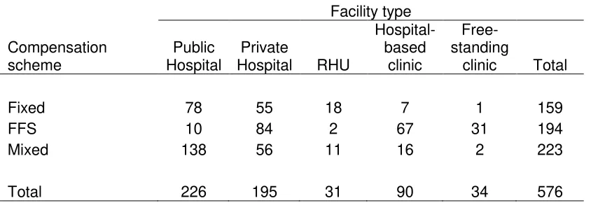
[image:18.612.72.494.466.611.2]Controlling for the selection, FFS and mixed payment increase vignette scores by about 10.99 percentage points and 3.3 percentage points, respectively. This supports our theoretical predictions that as long as the physician remains below the best level 𝑉̅ and as long as patient load is sufficiently high, FFS encourages quality compared to fixed payment. Mixed payment scheme also induces quality compared to fixed payment, albeit way lower than FFS. These positive coefficients indicate that there is still an incentive to improve quality. By looking at the cross-tabulation of payment schemes and facility types (see Table 4.4), we can see that while many physicians are already in either FFS or mixed, there are still a sizeable number of physicians who are operating in a fixed salary system, especially in public facilities (hospitals and RHUs). Hence, there could be a scope for introducing a mixed payment scheme to improve quality. At a policy perspective, Philhealth reimbursements may be a viable option.
Table 4.4: Cross-tabulation of compensation scheme and facility type (N=576)
Facility type
Compensation scheme
Public Hospital
Private
Hospital RHU
Hospital-based
clinic
Free-standing
clinic Total
Fixed 78 55 18 7 1 159
FFS 10 84 2 67 31 194
Mixed 138 56 11 16 2 223
Total 226 195 31 90 34 576
Source: OP Baseline Physician Survey, UPecon-Health Policy Development Program (HPDP)
18
We can also predict scores by facility type (public or private) while assuming actual values for the other explanatory variables. At fixed payment (that is, we set FFS and mixed to zero), the average score in public facilities is 39.3 percent while the score in private facilities is 37.4 percent. If we introduce FFS, scores in public facilities improved to 50.2 percent while scores in private facilities increased only up to 48.4 percent. However, if we introduce mixed payment, public facility physicians will only improve up to 42.6 percent and private facility physicians up to 40.7 percent. It appears then that the improvement in scores is more pronounced in public facilities over private facilities, although scores barely reached the 50 percent benchmark (except for FFS in public facilities).
We can also do the same simulation across vignette types. At the baseline, the scores are indeed lower for physicians answering the TB and pre-eclampsia vignettes at 25.6 percent and 24.4 percent, while the pneumonia and diarrhea physicians passed at 52.7 percent and 54.5 percent, respectively. When all physicians were to receive FFS, TB and pre-eclampsia vignette scores increased, but is still way below the passing mark at 36.6 percent and 35.4 percent, while pneumonia and diarrhea vignette scores improved. Scores did not increase as much under mixed. Again, this shows that while FFS and mixed payment schemes pose positive incentives to quality, they do not seem sufficient enough to increase scores up to or beyond the passing rate.
5. Conclusion
In this paper we have examined how payment schemes influence quality of care, measured by the vignettes. We constructed a simple model of physician quality, arguing that the different payment schemes yield different optimal work hours, which in turn affects total procedures and eventually quality scores. We predicted that, relative to fixed payment, FFS and mixed payment lead to higher quality. Using these predictions, we estimated the impact of payment schemes on quality by conducting multinomial treatment effects regression to account for endogeneity in the choice of payment scheme. We found evidence that relative to fixed payment, FFS and mixed payment yields higher vignette scores. On average, physicians under FFS score 11 percent higher than fixed payment while physicians under mixed score roughly 3 percent higher than mixed. We noted that notwithstanding these results, shifting all physicians to either FFS or mixed will barely lead to at least 50 percent in vignette scores. We accounted for endogeneity of payment scheme with location (urban-rural) as instrument. Selection of payment schemes is
also highly affected by physician’s age and, to some extent, specialization.
5.1. Policy notes
These results have shown plausible evidence that payment scheme policies can influence quality of care even accounting for incentives for self-selection into payment schemes. Our findings show that there is a stronger incentive in FFS to work harder and therefore provide services that input into quality.
In the Philippines, the Philippine Health Insurance Corporation (Philhealth) is the responsible
agency in financing providers through the facilities, in support of the Department of Health’s
19
to members and their dependents. Philhealth data8 shows that as of December 31, 2013, 1,761 hospitals were accredited from 1,670 in December 2012. Clinics offering primary care benefit packages rose to 2,538 from 1,805 in end-December 2012; maternity care packages 2,065 from 1,476; and TB-DOTS packages to 1,453 from 1,201. As more facilities become accredited, more physicians are likely to be entitled to receive FFS reimbursements. Along with the increasing Philhealth coverage across the country (through Kalusugan Pangkalahatan), demand for health care should also increase. Given the empirical results, providers in the public sector (i.e. fixed payment physicians) have the least incentive to provide quality care; nevertheless, providing them with opportunities to receive additional fees, for example, in the form of Philhealth reimbursements, moves them to a mixed system which will encourage them to provide quality services. With the growing number of accredited facilities and membership, Philhealth can be a potent mechanism to improve quality.
However, a system with working incentive mechanism and an effective quality monitoring mechanism should also be set in place. Along with Philhealth, the Professional Regulatory Commission and the Department of Health are the agencies in charge of monitoring entry in the profession and accreditation; however, we fall short in monitoring quality, with few and unreliable data and difficulty in assessing the use of practice guidelines in the private sector [WHO and DOH 2012]. Existence of regular quality monitoring system such as the Physician Quality Measure Reporting9 of the American Medical Association (AMA) could fill in gaps in quality data.
While children’s diseases, TB, and maternal deaths remain a significant health concern in the
Philippines, the inclusion of monitoring health-risk factors and emerging infectious diseases may also be considered for further research. Improved quality in monitoring of health risks can help in curbing non-communicable diseases, which is becoming a concern in both developed and developing countries, with 41 percent under-60 deaths coming from low-income economies [WHO 2011]. Notwithstanding measurement issues, low vignette scores should not be taken lightly by policy makers, especially with the results on TB and pre-eclampsia vignettes. If taken as a signal, this poor performance in health service delivery raises questions and issues on sufficiency and quality of health care providers, especially in poor and far-flung regions.
8 The 2013 Philhealth stats and charts can be downloaded from:
http://www.philhealth.gov.ph/about_us/statsncharts/snc2013.pdf. 2012 data can be found in: http://www.philhealth.gov.ph/about_us/statsncharts/snc2012.pdf.
9 See more at:
20
References
Arrow KJ [1963]. “Uncertainty and the Welfare Economics of Medical Care”. The American Economic Review 53(5): 941-973. Retrieved 28 July 2011 from
http://www.jstor.org/stable/1812044 .
Barnum H, Kutzin J, and Saxenian H [1995]. “Incentives and Provider Payment Methods”. The International Journal of Health Planning and Management 10(1): 23-45. Retrieved 27 May 2011. doi: 10.1002/hpm.4740100104
Brennan N and Shepard M [2010]. “Comparing Quality of Care in the Medicare Program”.
American Journal of Managed Care 2010 16(11): 841-848. Retrieved 3 Jan 2013 from:
http://www.ajmc.com/publications/issue/2010/2010-11-vol16-n11/ajmc_10nov_brennan841to848/4
Deb P and Trivedi PK [2006]. “Maximum simulated likelihood estimation of a negative binomial
regression model with multinomial endogenous treatment”. The Stata Journal 6, Number 2: 246-255. Retrieved 14 Dec 2013 from:
http://www.stata-journal.com/sjpdf.html?articlenum=st0105.
Deb P and Seck P [2009]. “Internal Migration, Selection Bias, and Human Development:
Evidence from Indonesia and Mexico”, UNDP Human Development Research Paper 2009/31. Retrieved 14 Dec 2013 from:
http://mpra.ub.uni-muenchen.de/19214/1/MPRA_paper_19214.pdf.
Demange G and Geoffard PY [2006]. “Reforming Incentive Schemes under Political
Constraints: The Physician Agency”. Annals of Economics and Statistics / Annales
d’Economie et de Statistique 83: 221-250. Retrieved 31 Jan 2012 from
http://www.jstor.org/stable/20079169.
Devlin RA and Sarma S [2008]. “Do Physician Remuneration Schemes Matter? The Case of
Canadian Family Physicians”. Journal of Health Economics 27(5): 1168-1181. Retrieved 4 Aug 2013 from:
http://artsandscience.usask.ca/economics/research/pdf/SSarmaRemuneration Paper2.pdf.
Dresselhaus TR, Peabody JW, Lee M, Glassman P, Luck J [2000]. “Measuring Compliance with Preventive Care Guidelines: A Comparison of Standardized Patients, Clinical Vignettes
and the Medical Record.” Journal of General Internal Medicine. Vol. 15 (11): 782-88.
Dresselhaus TR, Peabody JW, Luck J, and Bertenthal D [2004]. “An Evaluation of Vignettes for
Predicting Variation in the Quality of Preventive Care.” Journal of General Internal Medicine. Vol. 19; 1013-1018.
Ellis RP and McGuire TG [1986]. “Provider Behavior under Prospective Reimbursement: Cost
Sharing and Supply”. Journal of Health Economics 5: 129-151. Accessed 12 Dec 2011 from http://www.ppge.ufrgs.br/giacomo/arquivos/eco02072/ellis-mcguire-1986.pdf
21
CIRANO. Retrieved 31 Jan 2012 from http://www.cirpee.org/fileadmin/ documents/Cahiers_2010/CIRPEE10-34.pdf
Henning-Schmidt H, Selten R, and Wiesen D [2009]. “How Payment Systems Affect Physician’s Provision Behavior –An Experimental Investigation”. Discussion Paper 29/2009. Bonn Graduate School of Economics, University of Bonn. Retrieved 24 May 2012 from http://www.wiwi.uni-bonn.de/bgsepapers/bonedp/bgse03_2011.pdf
Kim C, Steers WN, Herman W, Mangione C, Venkat Narayan KM, and Ettner S [2007].
“Physician Compensation from Salary and Quality of Diabetes Care”. Society of General Internal Medicine 22: 448-452. Retrieved 15 Oct 2012. doi: 10.1007/s11606-007-0124-5.
Leonard KL, Masatu MC, and Vialou A [2007]. “Getting Doctors to Do Their Best: The Roles of
Ability and Motivation in Health Care Quality”. The Journal of Human Resources 42(3): 682-700. Retrieved 26 May 2011 from: http://www.jstor.org/stable/40057323.
Libby A and Thurston NK [2001]. “Effects of Managed Care Contracting on Physician Labor
Supply”. International Journal of Health Care Finance and Economics 1(2): 139-157. Retrieved 13 Oct 2011 from http://www.jstor.org/stable/3528869.
Luck J, Peabody JW, Dresselhaus TR, Lee M, and Glassman PA [2000]. “How Well Does Chart Abstraction Measure Quality? A Prospective Comparison of Standardized Patients with
the Medical Record.” The American Journal of Medicine, Vol.108: 642-649.
Maddala G [1983]. “Models with self-selectivity”. Limited-Dependent and Qualitative Variables in Economics. New York: Cambridge University Press. Retrieved 12 April 2013 from: http://public.econ.duke.edu/~vjh3/e262p_07S/readings/Maddala_Models_of_Self-Selectivity.pdf
Peabody JW, Luck J, Glassman PA, Dresselhaus TR, Lee M. [2000] “Comparison of Vignettes, Standardized Patients, and Chart Abstraction: A Prospective Validation Study of 3 Methods for Measuring Quality.” Journal of the American Medical Association, 283(13):
1715-1722.
Peabody JW, Tozija F, Munoz JA, Nordyke RJ and Luck J. [2004] “Using Vignettes to Compare
the Quality of Care Variation in Economically Divergent Countries.” Journal of Health Services Research. Vol. 39 (6): 03-0209r2. Retrieved from
www.ncbi.nlm.nih.gov/pmc/articles/PM1361107/?tool=pubmed
Peabody JW, Luck J, Glassman P, Jain S, Spell M and Hansen J. [2004] “Measuring the Quality
of Physician Practice by using Clinical Vignettes: a Prospective Validation Study.” Annals of Internal Medicine. Vol. 141(10): 771-80.
Peabody JW and Liu A. [2007]. “Comparing Quality in Disparate Settings Using Vignettes.”
Journal of Health Policy and Planning. Vol 22(5): 294-302.
Peabody JW, Florentino J, Shimkhada R, Solon O, Quimbo S. [2010]. “Quality Variation and its
22
Peabody JW, Shimkhada R, Quimbo S, Florentino J, Bacate MF, McCulloch C, Solon O. [2011].
“Financial Incentives and Measurement Improved Physicians Quality of Care in the Philippines.” Health Affairs. 10 (4) 773-81
Peabody JW, Shimkhada R, Quimbo S, Solon O, Javier X, McCulloch C. [2013]. “The Impact of Performance Incentives on Child Health Outcomes: Results from a Cluster Randomized
Controlled Trial in the Philippines.” Health Policy and Planning.
Phelps, CE [1992]. Health Economics. New York: Harper.
Quimbo S, Peabody JW, Shimkhada R, Woo K, Solon O [2008]. “Should we have confidence if a physician is accredited? A study of the relative impacts of accreditation and insurance
payments on quality of care in the Philippines”. Social Science & Medicine 67: 505-510.
Quimbo S, Peabody JW, Javier X, Shimkhada R, Solon O [2011]. “Pushing on a string: How policy might encourage private doctors to compete with the public sector on the basis of
quality”. Economics Letters 110, 101-103.
Rice T [1997]. “Physician Payment Policies: Impacts and Implications”. Annual Review of Public Health 18, 549-65.
Shane D and Trivedi P [2012]. “What Drives Differences in Health Care Demand? The Role of Health Insurance and Selection Bias”. Health, Econometrics and Data Group (HEDG) Working Papers, 12(09). Retrieved 14 Dec 2013 from
http://www.york.ac.uk/media/economics/documents/herc/wp/12_09.pdf.
Shimkhada R, Peabody JW, Quimbo S, Solon O. [2008]. “The Quality Improvement Demonstration Study: An Example of Evidence-Based Policy-Making in Practice.”
Health Research Policy and Systems. 25;6: 5.
Solon O, Woo K, Quimbo SA, Peabody JW, Florentino J, Shimkhada R. [2009]. “A Novel Method for Measuring Health Care System Performance: Experience from QIDS in the
Philippines,” Health Policy and Planning. 24(3):167-74
Thorton J and Eakin BK [1997]. “The Utility-Maximizing Self-Employed Physician”. The Journal of Human Resources 32 (1), 98-128. Retrieved 27 May 2011. doi: 10.2307/146242.
UPecon—Health Policy Development Program [2007]. Operational Plan Baseline Survey
[Dataset].
UPecon—Health Policy Development Program [2011]. Documentation of the HPDP Data Library. Unpublished manuscript.
World Health Organization [2011]. Noncommunicable Diseases Country Profile 2011. Retrieved 24 Jan 2013 from:
http://whqlibdoc.who.int/publications/2011/9789241502283_eng.pdf?ua=1
World Health Organization and Department of Health Philippines [2012]. Philippines Health Service Delivery Profile 2012. Retrieved from:
23