Exploiting real-time 3d visualisation to enthuse
students: a case study of using Visual Python in
engineering
Hans Fangohr
University of Southampton, Southampton SO17 1BJ, United Kingdom, [email protected]
Abstract. We describe our experience teaching programming and nu-merical methods to engineering students using Visual Python to exploit three dimensional real time visualisation. We describe the structure and content of this teaching module and evaluate the module after its de-livery. We find that the students enjoy being able to visualise physical processes (even if these have effectively only 1 or 2 spatial degrees of freedom) and this improves the learning experience.
1
Introduction
Computer controlled devices are used in virtually every area of science and tech-nology, and often carry business and safety critical [1, 2] roles. A substantial part of the work of engineers and scientist – both in academia and industry – is to use and to develop such devices and their controlling software. This requires design-ing and maintaindesign-ing software in subject areas includdesign-ing control, data analysis, simulations and design optimisation.
While students are generally given a broad education on mathematics which includes basics as well as advanced material, it is often the case that the sub-ject of software engineering is not taught. Instead, it is assumed that engineers and scientists will be able to pick up software engineering skills by learning a programming language (for example by reading a book) at the point of their career where software development is required. While this may be justified for very small programs it is inappropriate for larger projects. It is unrealistic to assume someone would be able to master solving differential equations if they have only learned about polynomials (but not differential operators).
There are two cost factors attached to not having appropriate software engi-neering skills: (i) often not the most efficient approach to solve a given problem is chosen, and (ii) the written code is unlikely to be re-usable.
In section 2 we explain what motivates us to use Visual Python. Section 3 reports from teaching a module using Visual Python, and evaluates feedback from students and teachers. We suggest that virtual reality tools should be used more broadly in section 4 and close with a summary in section 5.
2
Background
2.1 What is Python?
Python [3] is an interpreted, interactive, object-oriented programming language. It is often compared to Tcl, Perl, Scheme or Java and combines remarkable power with very clear syntax. It has been argued that Python is an excellent choice of programming language for beginners both in computer science [4] and in other disciplines [5–7].
2.2 What is Visual Python?
Visual Python (VPython) [8] is a 3d graphics system that is an extension of the Python language. Its main usage has been in the area of demonstration of physical systems in physics, chemistry, and engineering. VPython was initially written by David Scherer under the supervision of Bruce Sherwood and Ruth Chabay and is is released under the GNU Public License.
2.3 Motivation for using Visual Python
Scientists in all stages of their career like solving puzzles: curiosity and the strong desire to understand the world drive them. We argue that this is not too distant from the keen young student who might like to play computer games: here, too, the player needs to solve a puzzle (to win the game). Some of the attractiveness of computer games stems from (i) their interactivity and (ii) the real time virtual reality graphics.
It is well known that the learning process is more successful if learners en-joy the learning activity and even more so if they start to explore the subject following their own ideas. We therefore strive to inspire the learners’ imagina-tion and provide them tools that encourage experimentaimagina-tion in computaimagina-tional science. We pick up the two points made above and make computational science (i) interactive and (ii) employ virtual reality graphics.
In a historical context, 2d visualisation has been introduced into teaching programming (and mathematics) via the “turtle” within the LOGO program-ming language more than 25 years ago [9]. More recently, “Alice” [10] provides an environment which allows the student to be the director of a movie or the creator of a video game and to create highly sophisticated 3d scenes with very little effort. Again, the aim is to allow traditional programming concepts to be more easily taught and more readily understood [11].
We have chosen Visual Python because it offers true 3d graphics (with simple building blocks such as spheres, boxes, cones etc), it is extremely easy to learn, and it is sufficiently “serious” to be used in real-life tasks in engineering and science.
3
Case study
3.1 Module layout and structure
In 2004/2005 the 85 second year Aerospace students at the University of Southamp-ton were taught a computing module [12] as outlined and evaluated in this sec-tion.
The course consists of 12 lectures (one a week) and 6 associated practical sessions in a computer laboratory equipped with standard PCs running MS Windows. The practical laboratories take place every two weeks, last 3 hours, and every student is doing one self-paced assignments using their computer. Demonstrators are available in the laboratories (approximately one demonstrator per 10 students) to provide help if necessary. In each of the first four laboratory sessions students have to complete one self-paced assignment. When completed, they are asked to explain their work (both computer programmes and any other notes) to a demonstrator in a mini-viva between one demonstrator and one student lasting between 10 and 15 minutes (in front of the student’s computer). The fifth assignment is slightly larger and students have to submit a written report to be marked off-line by the lecturer (without the student being present). The fifth assignment is also used as a report writing exercise.
3.2 Content
Students’ background in numerical methods: This module is preceded by 12 lectures (each lasting 45 minutes) providing a theoretical introduction to numerical methods (including elementary linear algebra, root finding, numerical integration of ordinary differential equations) without practical exercises. Due to time-tabling constraints it has not been possible to combine the more problem-solving based module described here with these theory lessons (although this is desirable).
A sphere at positionr= (rx, ry, rz)of massm= 1kgis sub-ject to a horizontal forceFspring = (−krx,0,0)and to a verti-cal force due to gravityFgrav= (0,−mg,0). The initial posi-tion isr(t0) = (3,5,0)m, initial velocity v(t0) = (0,0,0)m/s
and k = 5N/m. Compute the time development of the sys-tem, assuming that the sphere will bounce elastically when it touches the ground atry= 0.
Fig. 1. (Left) An example problem and (right) a snapshot of an animation of the solution. The faint line which starts filling a rectangular is the trajectory of the sphere and updated as the sphere moves.
year. This included four computer based exercises introducing fundamental con-cepts such as if-then statements, for-loops and functions on a very basic level.
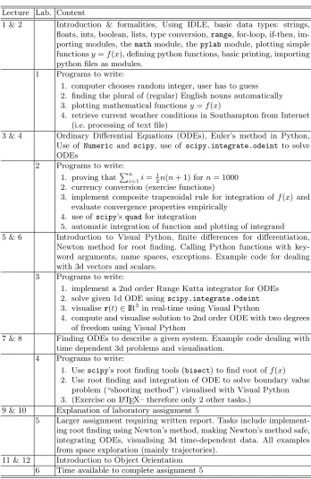
The content of this module is given in table 1 and ordered by lectures (numbered from 1 to 12) and laboratory sessions (numbered from 1 to 6).
As can be seen, we have combined a repetition of numerical methods with the introduction of the Python programming language (laboratories 1 and 2) and Visual Python (laboratories 3, 4 and 5).
Required Software: Apart fromPython[3], we requireNumeric[14],Scientific Python [15], Pylab (formerlyMatplotlib) [16] and Visual Python [8]. All of these can be installed on the major three platforms MS Windows, Linux and Mac OS X.
For MS Windows, we have found the ”Enthought Python” edition [17] of great value which bundles Python with all the extra packages we need (apart from Visual Python which can be installed afterwards) and simplifies the in-stallation of the software both for IT personnel at the university as well as for students at home.
3.3 Results and discussion
A visualisation example is shown in figure 1 and has been created by the program shown in figure 2. It is outside the scope of this paper to explain the workings of the program detail. However, hopefully this demonstrates that it encourages experimentation to support understanding the system. (This problem could be tackled by the students in laboratory session 4).
Lecture Lab. Content
1 & 2 Introduction & formalities, Using IDLE, basic data types: strings, floats, ints, boolean, lists, type conversion,range, for-loop, if-then, im-porting modules, themathmodule, thepylabmodule, plotting simple functionsy=f(x), defining python functions, basic printing, importing python files as modules.
1 Programs to write:
1. computer chooses random integer, user has to guess 2. finding the plural of (regular) English nouns automatically 3. plotting mathematical functionsy=f(x)
4. retrieve current weather conditions in Southampton from Internet (i.e. processing of text file)
3 & 4 Ordinary Differential Equations (ODEs), Euler’s method in Python, Use of Numeric and scipy, use of scipy.integrate.odeint to solve ODEs
2 Programs to write: 1. proving thatPni=1i=
1
2n(n+ 1) forn= 1000 2. currency conversion (exercise functions)
3. implement composite trapezoidal rule for integration of f(x) and evaluate convergence properties empirically
4. use of scipy’squadfor integration
5. automatic integration of function and plotting of integrand 5 & 6 Introduction to Visual Python, finite differences for differentiation,
Newton method for root finding. Calling Python functions with key-word arguments, name spaces, exceptions. Example code for dealing with 3d vectors and scalars.
3 Programs to write:
1. implement a 2nd order Runge Kutta integrator for ODEs 2. solve given 1d ODE usingscipy.integrate.odeint 3. visualiser(t)∈IR3 in real-time using Visual Python
4. compute and visualise solution to 2nd order ODE with two degrees of freedom using Visual Python
7 & 8 Finding ODEs to describe a given system. Example code dealing with time dependent 3d problems and visualisation.
4 Programs to write:
1. Usescipy’s root finding tools (bisect) to find root off(x) 2. Use root finding and integration of ODE to solve boundary value
problem (“shooting method”) visualised with Visual Python 3. (Exercise on LATEX– therefore only 2 other tasks.)
9 & 10 Explanation of laboratory assignment 5
5 Larger assignment requiring written report. Tasks include implement-ing root findimplement-ing usimplement-ing Newton’s method, makimplement-ing Newton’s method safe, integrating ODEs, visualising 3d time-dependent data. All examples from space exploration (mainly trajectories).
[image:5.612.134.482.59.594.2]11 & 12 Introduction to Object Orientation 6 Time available to complete assignment 5
from Numeric import array, concatenate import scipy, visual
def rhs(y,t):
"""function that returns dy/dt(y,t) for system of ODE""" vx, vy, vz, rx, ry, rz = y
mass = 1.0 #mass of object in kg
g = 9.81 #acceleration from Earth in N/kg F_grav = array([0,-g, 0])*mass
spring_x = 0 #spring equilibrium at x=0 (in m) k = 5 #spring stiffness in N/m
F_spring = k*array([spring_x-rx,0,0]) dvdt = (F_spring + F_grav)/mass drdt = (vx,vy,vz)
return concatenate([dvdt,drdt])
#main program starts here
r = array([3,5,0]) #initial position of object in m v = array([0,0,0]) #initial velocity of object in m/s
t = 0 #current time in s
dt = 1/30.0 #time step in seconds, to match framerate
#visualisation
visual.scene.autoscale = False #don’t zoom in and out visual.scene.center = (0,3,0) #focus camera it this point
base = visual.box(pos=(0,-0.5,0), length=10, height=0.1, width=4) pole_x = -5 #position arbitrarily chosen
cylinder= visual.cylinder(pos=(pole_x,-1,0),axis=(0,7,0),radius=0.3) ball = visual.sphere(pos=r,radius=0.5,color=visual.color.white) spring = visual.helix(pos=r,axis=(pole_x-r[0],-1,0),thickness=0.1) path = visual.curve() #initiate drawing path of trajectory
while True: #infinite time loop starts y = concatenate([v,r])
#integrate the system from time t to t+dt
y = scipy.integrate.odeint(rhs,y,array([t,t+dt])) t = t + dt #advance time
v = y[-1,0:3] #extract last row from output from odeint r = y[-1,3:6] #for visualisation
if r[1] < 0: #if below base plate
v[1] = -v[1] #then reverse velocity (elastic bounce)
visual.rate(30) #visualisation: keep frame rate constant ball.pos = r # update position of ball path.append(r) # update trace
spring.pos=r # update spring head spring.axis = (pole_x-r[0],0,0) #update spring tail
Feedback from the teacher includes the following observations:
⊲ The overall reception of the module was very good, in particular taking into account that within the student body the subject of “computing” is often regarded as difficult and boring.
⊲ A number of students wrote programs unrelated to the module and in their spare time because they enjoyed the process. These included an analog clock (using Visual Python for the central knob, hands and hour-ticks) and a visualisation of the orbits of planets within the solar system.
⊲ Visual Python can render its 3d graphics for coloured anaglyph glasses (here red-cyan) with the following commandvisual.scene.stereo=’redcyan’. This allows seeing the scene with spacial depth and simple glasses can be bought for about one US dollar or Euro. This proved popular with students and has clearly boosted the motivation.
⊲ This module was previously taught in Matlab [13] using a similar content and structure. However, it turned out that it was not possible to simple ’re-write’ the learning materials and lectures to be delivered in Python. For example, previously a complete laboratory session was used to introduce the correct syntax (in Matlab) to pass a function to a function. This is required if, say, general purpose integrators are written. With Python, a function is an object as is any other object, and can be passed to a function and then used as if it was defined elsewhere in the code (see also [6]). This change immediately freed up several hours of time in the laboratory sessions and allowed us to proceed further in terms of numerical methods.
⊲ The real-time integration of ordinary differential equations (ODEs) and the real-time display of the simulated process allows students to gain a deeper understanding of the physical process in comparison to looking at 2d graphs showing the displacement of an object against time. We are not able to quan-tify this but have got the impression that this was supporting the learning process.
4
Outlook
There are a number of topics in Physics [18], Mathematics [19] and elsewhere which could benefit from being taught together with virtual reality tools such as Visual Python. For example, when the topic of Vibrations (or “normal modes”) is taught, the lecturer often demonstrates with an experimental set up how energy transfers from one pendulum to another when these are coupled by a spring. The students could be given a Visual Python program which allows to repeat this experiment and to vary the initial conditions and system parameters as much as they like outside the lecture.
5
Summary
In summary we describe our experiences of using Visual Python to enthuse engi-neering students when learning the fundamental concepts of software engiengi-neering and programming. Feedback from students and staff shows that the real-time virtual reality environment has improved the learning experience. We link exer-cises to other parts of their curriculum (such as ordinary differential equations) to contextualise the new skills. We argue that there are a number of areas which naturally allow (and would benefit from) the integration of computation and visualisation into the existing curriculum.
References
1. Je’ze’quel, J.M., Meyer, B.: Design by contract: The lessons of Ariane. IEEE Computer30(2) (1997) 129–130
2. Leveson, N.G., Turner, C.S.: An investigation of the Therac-25 accidents. IEEE Computer26(7) (1993) 18–41
3. van Rossum, G.: Python tutorial. Centrum voor Wiskunde en Informatica (CWI), Amsterdam. (1995)http://www.python.org.
4. Downey, A., Elkner, J., Meyers, C.: How to Think Like a Com-puter Scientist: Learning with Python. Green Tea Press (2002) http://www.greenteapress.com/thinkpython/html.
5. Donaldson, T.: Python as a first programming language for every-one. In: Western Canadian Conference on Computing Education. (2003) http://www.cs.ubc.ca/wccce/Program03/papers/Toby.html.
6. Fangohr, H.: A comparison of C, Matlab and Python as teaching languages in engineering. Lecture Notes on Computational Science3039(2004) 1210–1217 7. Roberts, S., Gardner, H., Press, S., Stals, L.: Teaching computational science using
vpython and virtual reality. Lecture Notes on Computational Science3039(2004) 1218–1225
8. Scherer, D., Sherwood, B., Chabay, R.: (2005)http://www.vpython.org. 9. Papert, S.: Mindstorms: Children, Computers and Powerful Ideas. Prentice Hall
Europe (1980)
10. Carnegie Mellon University: (2005)http://www.alice.org.
11. Dann, W., Cooper, S., Pausch, R.: Learning to Program with Alice. Prentice Hall (2005)
12. Fangohr, H.: Computing module SESA2006, Aerospace Engineering, University of Southampton (2004) The complete learning materials are available from the author on request.
13. The Mathworks: Matlab (2005)www.mathworks.com. 14. http://numeric.scipy.org.
15. http://scipy.org.
16. http://matplotlib.sourceforge.net. 17. http://www.enthought.com/python.
18. Chabay, R.W., Sherwood, B.A.: Matter and Interactions: Modern Mechanics and Electric and Magnetic Interactions. John Wiley and Sons (2003)