Multiple-stream Language Models for Statistical Machine Translation
Abby Levenberg
Dept. of Computer Science University of Oxford
Miles Osborne
School of Informatics University of Edinburgh
David Matthews
School of Informatics University of Edinburgh
Abstract
We consider using online language models for translating multiple streams which naturally arise on the Web. After establishing that us-ing just one stream can degrade translations on different domains, we present a series of simple approaches which tackle the problem of maintaining translation performance on all streams in small space. By exploiting the dif-fering throughputs of each stream and how the decoder translates prior test points from each stream, we show how translation perfor-mance can equal specialised, per-stream lan-guage models, but do this in a single lanlan-guage model using far less space. Our results hold even when adding three billion tokens of addi-tional text as a background language model.
1 Introduction
There is more natural language data available today than there has ever been and the scale of its produc-tion is increasing quickly. While this phenomenon provides the Statistic Machine Translation (SMT) community with a potentially extremely useful re-source to learn from, it also brings with it nontrivial computational challenges of scalability.
Text streams arise naturally on the Web where millions of new documents are published each day in many different languages. Examples in the stream-ing domain include the thousands of multilstream-ingual websites that continuously publish newswire stories, the official proceedings of governments and other bureaucratic organisations, as well as the millions of “bloggers” and host of users on social network services such as Facebook and Twitter.
Recent work has shown good results using an in-coming text stream as training data for either a static or online language model (LM) in an SMT setting (Goyal et al., 2009; Levenberg and Osborne, 2009). A drawback of prior work is the oversimplified sce-nario that all training and test data is drawn from the same distribution using a single, in-domain stream. In a real world scenario multiple incoming streams are readily available and test sets from dissimilar do-mains will be translated continuously. As we show, using stream data from one domain to translate an-other results in poor average performance for both streams. However, combining streams naively to-gether hurts performance further still.
In this paper we consider this problem of multiple stream translation. Since monolingual data is very abundant, we focus on the subtask of updating an on-line LM using multiple incoming streams. The chal-lenges in multiple stream translation include dealing with domain differences, variable throughput rates (the size of each stream per epoch), and the need to maintain constant space. Importantly, we impose the key requirement that our model match transla-tion performance reached using the single stream ap-proach on all test domains.
We accomplish this using the n-gram history of prior translations plus subsampling to maintain a constant bound on memory required for language modelling throughout all stream adaptation. In par-ticular, when considering two test streams, we are able to improve performance on both streams from an average (per stream) BLEU score of 39.71 and 37.09using a single stream approach (Tables 2 and 3) to an average BLEU score of41.28and42.73 us-ing multiple streams within a sus-ingle LM usus-ing equal memory (Tables 6 and 7). We also show additive
provements using this approach when using a large background LM consisting of over one billion n -grams. To our knowledge our approach is the first in the literature to deal with adapting an online LM to multiple streams in small space.
2 Previous Work
2.1 Randomised LMs
Randomised techniques for LMs from Talbot and Osborne (2007) and Talbot and Brants (2008) are currently industry state-of-the-art for fitting very large datasets into much smaller amounts of mem-ory than lossless representations for the data. Instead of representing then-grams exactly, the randomised representation exchanges a small, one-sided error of false positives for massive space savings.
2.2 Stream-based LMs
An unbounded text stream is an input source of natu-ral language documents that is received sequentially and so has an implicit timeline attached. In Leven-berg and Osborne (2009) a text stream was used to initially train and subsequently adapt an online, ran-domised LM (ORLM) with good results. However, a weakness of Levenberg and Osborne (2009) is that the experiments were all conducted over a single in-put stream. It is an oversimplification to assume that all test material for a SMT system will be from a sin-gle domain. No work was done on the multi-stream case where we have more than one incoming stream from arbitrary domains.
2.3 Domain Adaptation for SMT
Within MT there has been a variety of approaches dealing with domain adaptation (for example (Wu et al., 2008; Koehn and Schroeder, 2007)). Our work is related to domain adaptation but differs in that we are not skewing the distribution of an out-of-domain LM to accommodate some test data for which we have little or no training data for. Rather, we have varying amounts of training data from all the do-mains via the incoming streams and the LM must account for each domain appropriately. However, known domain adaptation techniques are potentially applicable to multi-stream translation as well.
3 Multiple Streams and their Properties
Any source that provides a continuous sequence of natural language documents over time can be thought of as an unbounded stream which is time-stamped and access to it is given in strict chronolog-ical order. The ubiquity of technology and the In-ternet means there are many such text streams avail-able already and their number is increasing quickly. For SMT, multiple text streams provide a potentially abundant source of new training data that may be useful for combating model sparsity.
Of primary concern is building models whose space complexity is independent of the size of the incoming stream. Allowing unbounded memory to handle unbounded streams is unsatisfactory. When dealing with more than one stream we must also consider how the properties of single streams inter-act in a multiple stream setting.
Every text stream is associated with a particular domain. For example, we may draw a stream from a newswire source, a daily web crawl of new blogs, or the output of a company or organisation. Obvi-ously the distribution over the text contained in these streams will be very different from each other. As is well-known from the work on domain adaptation throughout the SMT literature, using a model from one domain to translate a test document from an-other domain would likely produce poor results.
Each stream source will also have a different rate of production, or throughput, which may vary greatly between sources. Blog data may be received in abundance but the newswire data may have a sig-nificantly lower throughput. This means that the text stream with higher throughput may dominate and overwhelm the more nuanced translation options of the stream with less data in the LM during decod-ing. This is bad if we want to translate well for all domains in small space using a single model.
4 Multi-Stream Retraining
…
input stream 1 input stream 2
input stream K
LM 1
LM 2
LM 3
Naive Combination Approach
[image:3.612.74.296.58.156.2]new epoch new epoch
Figure 1: In the naive approach allKstreams are simply combined into a single LM for each new epoch encoun-tered.
Given an incoming number K of unbounded streams over a potentially infinite timelineT, with
t⊂T an epoch or windowed subset of the timeline, the full set ofn-grams in all K streams over allT
is denoted withS. By Stwe denoten-grams from all K streams andSkt, k ∈ [1, K], as then-grams in the kth stream over epocht. Since the streams are unbounded, we do not have access to all then -grams inSat once. Instead we selectn-grams from each stream Skt ⊂ S. We define the collection of
n-grams encoded in the LM at time t over all K
streams as Ct. Initially, at time t = 0 the LM is composed of then-grams in the stream soC0 =S0. Since it is unsatisfactory to allow unbounded memory usage for the model and more bits are needed as we see more novel n-grams from the streams, we enforce a memory constraint and use an adaptation scheme to delete n-grams from the LMCt−1before adding any newn-grams from the streams to get the current n-gram set Ct. Below we describe various approaches of updating the LM with data from the streams.
4.1 Naive Combinations
Approach The first obvious approach for an online LM using multiple input streams is to simply store all the streams in one LM. That is, n-grams from all the streams are only inserted into the LM once and their stream specific counts are combined into a single value in the composite LM.
Modelling the Stream In the naive case we retrain the LMCt in full at epochtusing all the new data from the streams. We have simply
Ct= K [
k=1
Skt (1)
stream 1 LM 1
stream 1 LM 2
stream 1 LM 3 input stream 1
stream 2 LM 1
stream 2 LM 2
stream 2 LM 3 input stream 2
…
stream K LM 1
stream K LM 2
stream K LM 3 input stream K
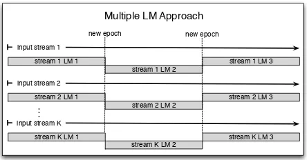
Multiple LM Approach
[image:3.612.316.538.59.175.2]new epoch new epoch
Figure 2: Each stream1. . . Kgets its own stream-based LM using the multiple LM approach.
where each of theKstreams is combined into a sin-gle model and then-grams counts are merged lin-early. Here we carry non-grams over from the LM
Ct−1from the previous epoch. The space needed is the number of unique n-grams present in the com-bined streams for each epoch.
Resulting LM To query the resulting LMCt dur-ing decoddur-ing with a testn-gramwin= (wi, . . . , wn) we use a simple smoothing algorithm called Stupid Backoff (Brants et al., 2007). This returns the probability of ann-gram as
P(wi|wii−1 −n+1) :=
Ct(wii
−n+1)
Ct(w i−1 i
−n+1)
ifCt(wii−n+1)>0
αP(wi|w i−1
i−n+2) otherwise
(2)
whereCt(.)denotes the frequency count returned by the LM for ann-gram andαis a backoff parameter. The recursion ends once the unigram is reached in which case the probability isP(wi) :=wi/N where
N is the size of the current training corpus.
4.2 Weighted Interpolation
Approach An improved approach to using multi-ple streams is to build a separate LM for each stream and using a weighted combination of each during decoding. Each stream is stored in isolation and we interpolate the information contained within each during decoding using a weighting on each stream. Modelling the Stream Here we model the streams by simply storing each stream at time t in its own LM soCkt=Sktfor each streamSk. Then the LM after epochtis
Ct={C1t, . . . , CKt}.
We use more space here than all other approaches since we must store eachn-gram/count occurring in each stream separately as well as the overhead in-curred for each separate LM in memory.
Resulting LM During decoding, the probability of a testn-gram wn
i is a weighted combination of all the individual stream LMs. We can write
P(wni) := K X
k=1
fkPCkt(w n
i) (3)
where we query each of the individual LMsCktto get a score from each LM using Equation 2 and combine them together using a weighting fk spe-cific to each LM. Here we impose the restriction on the weights thatPKk=1fk = 1. (We discuss specific weight selections in the next section.)
By maintaining multiple stream specific LMs we maintain the particular distribution of the individual streams. This keeps the more nuanced translations from the lower throughput streams available during decoding without translations being dominated by a stream with higher throughput. However using mul-tiple distinct LMs is wasteful of memory.
4.3 Combining Models via History
Approach We want to combine the streams into a single LM using less memory than when storing each stream separately but still achieve at least as good a translation for each test point. Naively com-bining the streams removes stream specific transla-tions but using the history ofn-grams selected by the decoder during the previous test point in the stream was done in Levenberg and Osborne (2009) for the
single stream case with good results. This is appli-cable to the multi-stream case as well.
Modelling the Stream For multiple streams and epocht >0we model the stream combination as
Ct=fT(Ct−1)∪
K [
k=1
(Skt). (4)
where for each epoch a selected subset of the previ-ousn-grams in the LMCt−1 is merged with all the newly arrived stream data to create the new LM set
Ct. The parameterfT denotes a function that filters over the previous set of n-grams in the model. It represents the specific adaptation scheme employed and stays constant throughout the timelineT. In this work we consider any n-grams queried by the de-coder in the last test point as potentially useful to the next point. Since all of the n-grams St in the stream at timetare used the space required is of the same order of complexity as the naive approach. Resulting LM Since all the n-grams from the streams are now encoded in a single LMCtwe can query it using Equation 2 during decoding. The goal of retraining using decoding history is to keep use-fuln-grams in the current model so a better model is obtained and performance for the next transla-tion point is improved. Note that making use of the history for hypothesis combination is theoretically well-founded and is the same approach used here for history based combination. (Mansour et al., 2008)
4.4 Subsampling
Approach The problem of multiple streams with highly varying throughput rates can be seen as a type of class imbalance problem in the machine learning literature. Given a binary prediction problem with two classes, for instance, the imbalance problem oc-curs when the bulk of the examples in the training data are instances of one class and only a much smaller proportion of examples are available from the other class. A frequently used approach to bal-ancing the distribution for the statistical model is to use random under sampling and select only a sub-set of the dominant class examples during training (Japkowicz and Stephen, 2002).
…
input stream 1 input stream 2
input stream K
LM 1
LM 2 + (subset of LM 1)
LM 3 + (subset of LM 2)
History Combination Approach
new epoch new epoch
[image:5.612.330.525.58.112.2]SMT Decoder
Figure 3: Using decoding history all the streams are com-bined into a unified LM.
subsampling selection scheme directly to the incom-ing streams to balance each stream’s contribution in the final LM. Note that subsampling is also related to weighting interpolation. Since all returned LM scores are based on frequency counts of then-grams and their prefixes, taking a weighting on a full prob-ability of ann-gram is akin to having fewer counts of then-grams in the LM to begin with.
Modelling the Stream To this end we use the weighted function parameterfkfrom Equation 3 to serve as the sampling probability rate for accepting an n-gram from a given stream k. The sampling rate serves to limit the amount of stream data from a stream that ends up in the model. ForK > 1we have
Ct=fT(Ct−1)∪
K [
k=1
fk(Skt) (5)
wherefkis the probability a particularn-gram from stream Sk at epoch t will be included in Ct. The adaptation functionfT remains the same as in Equa-tion 4. The space used in this approach is now de-pendent on the ratefkused for each stream.
Resulting LM Again, since we obtain a single LM from all the streams, we use Equation 2 to get the probability of ann-gram during decoding.
The subsampling method is applicable to all of the approaches discussed in this section. However, since we are essentially limiting the amount of data that we store in the final LM we can expect to take a per-formance hit based on the rate of acceptance given by the parameters fk. By using subsampling with the history combination approach we obtain good performance for all streams in small space.
Stream 1-grams 3-grams 5-grams
EP 19K 520K 760K
GW (xie) 120K 3M 5M
[image:5.612.74.298.58.175.2]RCV1 630K 21M 42M
Table 1: Sample statistics of uniquen-gram counts from the streams from epoch 2 of our timeline. The throughput rate varies a lot between streams.
5 Experiments
Here we report on our SMT experiments with multi-ple streams for translation using the approaches out-lined in the previous section.
5.1 Experimental Setup
The SMT setup we employ is standard and all re-sources used are publicly available. We translate from Spanish into English using phrase-based de-coding with Moses (Koehn and Hoang, 2007) as our decoder. Our parallel data came from Europarl.
We use three streams (all are timestamped): RCV1 (Rose et al., 2002), Europarl (EP) (Koehn, 2003), and Gigaword (GW) (Graff et al., 2007). GW is taken from six distinct newswire sources but in our initial experiments we limit the incoming stream from Gigaword to one of the sources (xie). GW and RCV1 are both newswire domain streams with high rates of incoming data whereas EP is a more nu-anced, smaller throughput domain of spoken tran-scripts taken from sessions of the European Parlia-ment. The RCV1 corpus only spans one calender year from October, 1996 through September, 1997 so we selected only data in this time frame from the other two streams so our timeline consists of the same full calendar year for all streams.
For this work we use the ORLM. The crux of the ORLM is an online perfect hash function that pro-vides the ability to insert and delete from the data structure. Consequently the ORLM has the abil-ity to adapt to an unbounded input stream whilst maintaining both constant memory usage and error rate. All the ORLMs were 5-gram models built with training data from the streams discussed above and used Stupid Backoff smoothing forn-gram scoring (Brants et al., 2007). All results are reported using the BLEU metric (Papineni et al., 2001).
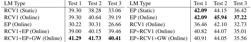
LM Type Test 1 Test 2 Test 3 RCV1 (Static) 39.30 38.28 33.06 RCV1 (Online) 39.30 40.64 39.19 EP (Online) 30.22 30.31 26.66 RCV1+EP (Online) 39.00 40.15 39.46 RCV1+EP+GW (Online) 41.29 41.73 40.41
Table 2: Results for the RCV1 test points. RCV1 and GW streams are in-domain and EP is out-of-domain. Transla-tion results are improved using more stream data since mostn-grams are in-domain to the test points.
from both the RCV1 and EP stream’s timeline for a total of six test points. This divided the streams into three epochs, and we updated the online LM using the data encountered in the epoch prior to each translation point. Then-grams and their counts from the streams are combined in the LM using one of the approaches from the previous section.
Using the notation from Section 4 we have the RCV1, EP, and GW streams described above and
K = 3as the number of incoming streams from two distinct domains (newswire and spoken dialogue). Our timelineT is one year’s worth of data split into three epochs, t ∈ {1,2,3}, with test points at the end of each epocht. Since we have no test points from the GW stream it acts as a background stream for these experiments.1
5.2 Baselines and Naive Combinations
In this section we report on our translation exper-iments using a single stream and the naive linear combination approach with multiple incoming data streams from Section 4.1.
Using the RCV1 corpus as our input stream we tested single stream translation first. Here we are replicating the experiments from Levenberg and Os-borne (2009) so both training and test data comes from a single in-domain stream. Results are in Table 2 where each row represents a different LM type.
RCV1 (Static) is the traditional baseline with no
adaptation where we use the training data for the first epoch of the stream. RCV1 (Online) is the online LM adapted with data from the in-domain stream. Confirming the previous work we get improvements
1
A background stream is one that only serves as training data for all other test domains.
[image:6.612.70.552.59.141.2]LM Type Test 1 Test 2 Test 3 EP (Static) 42.09 44.15 36.42 EP (Online) 42.09 45.94 37.22 RCV1 (Online) 36.46 42.10 32.73 EP+RCV1 (Online) 40.82 44.07 35.01 EP+RCV1+GW (Online) 40.91 44.05 35.56
Table 3: EP results using in and out-of-domain streams. The last two rows show that naive combination gets poor results compared to single stream approaches.
when using an online LM that incorporates recent data against a static baseline.
We then ran the same experiments using a stream generated from the EP corpus. EP consists of the proceedings of the European Parliament and is a sig-nificantly different domain than the RCV1 newswire stream. We updated the online LM using n-grams from the latest stream epoch before translating each in-domain EP test set. Results are in Table 3 and fol-low the same naming convention as Table 2 (except now in-domain is EP and out-of-domain is RCV1).
Using a single stream we also cross tested and translated each test point using the online LM adapted on the out-of-domain stream. As expected, translation performance decreases (sometimes dras-tically) in this case since the data of the out-of-domain stream are not suited to the out-of-domain of the current test point being translated.
Weighting Test 1 Test 2 Test 3
.33R+.33E +.33G 38.97 39.78 35.66
.50R+.25E +.25G 39.59 40.40 37.22
.25R+.50E +.25G 36.57 38.03 34.23
[image:7.612.78.295.58.126.2].70R+ 0.0E +.30G 40.54 41.46 39.23
Table 4: Weighted LM interpolation results for the RCV1 test points whereE =Europarl, R =RCV1, andG =
Gigaword (xie).
points due to the addition of in-domain data but the EP test performance still suffers.
This highlights why naive combination is unsat-isfactory. While using more in-domain data aids in the translation of the newswire tests, for the EP test sets, naively combining the n-grams from all streams means the hypotheses the decoder selects are weighted heavily in favor of the out-of-domain data. As the out-of-domain stream’s throughput is significantly larger it swamps the model.
5.3 Interpolating Weighted Streams
Straightforward linear stream combination into a single LM results in degradation of translations for test points whose in-domain training data is drawn from a stream with lower throughput than the other data streams. We could maintain a separate MT sys-tem for each streaming domain but intuitively some combination of the streams may benefit average per-formance since using all the data available should benefit test points from streams with low through-put. To test this we used an alternative approach de-scribed in Section 4.2 and used a weighted combi-nation of the single stream LMs during decoding.
We tested this approach using our three streams: RCV1, EP and GW (xie). We used a separate ORLM for each stream and then, during testing, the result returned for ann-gram queried by the decoder was a value obtained from some weighted interpola-tion of each individual LM’s score for thatn-gram. To get the interpolation weights for each streaming LM we minimised the perplexity of all the mod-els on held-out development data from the streams.
2 Then we used the corresponding stream specific
2Due to the lossy nature of the encoding of the ORLM
means that the perplexity measures were approximations. Nonetheless the weighting from this approach had the best per-formance.
Weighting Test 1 Test 2 Test 3
.33E+.33R+.33G 40.75 45.65 35.77
.50E+.25R+.25G 41.46 46.37 36.94
.25E+.50R+.25G 40.57 44.90 35.77
.70E+.20R+.10G 42.47 46.83 38.08
Table 5: EP results in BLEU for the interpolated LMs.
weights to decode the test points from that domain. Results are shown in Tables 4 and 5 using the weighting scheme described above plus a selec-tion of random parameter settings for comparison. Using the notation from Section 4.2, a caption of “.5R+.25E+.25G”, for example, denotes a weight-ing offRCV1 = 0.5for the scores returned from the
RCV1 stream LM whilefEP andfGW = 0.25 for the EP and GW stream LMs.
The weighted interpolation results suggest that while naive combination of the streams may be mis-guided, average translation performance can be im-proved upon when using more than a single in-domain stream. Comparing the best results in Tables 2 and 3 to the single stream baselines in Tables 4 and 5 we achieve comparable, if not improved, transla-tion performance for both domains. This is espe-cially true for test domains such as EP which have low training data throughput from the stream. Here adding some information from the out-of-domain stream that contains a lot more data aids signifi-cantly in the translation of in-domain test points.
However, the optimal weighting differs between each test domain. For instance, the weighting that gives the best results for the EP tests results in much poorer translation performance for the RCV1 test points requiring us to track which stream we are decoding and then select the appropriate weighting. This adds unnecessary complexity to the SMT sys-tem. And, since we store each stream separately, memory usage is not optimal using this scheme.
5.4 History and Subsampling
For space efficiency we want to represent multi-ple streams non-redundantly instead of storing each stream/domain in its own LM. Here we report on experiments using both the history combination and subsampling approaches from Sections 4.3 and 4.4.
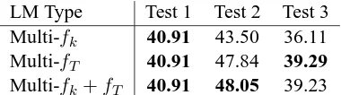
[image:7.612.316.535.59.126.2]LM Type Test 1 Test 2 Test 3 Multi-fk 41.19 41.73 39.23 Multi-fT 41.29 42.23 40.51 Multi-fk+fT 41.19 42.52 40.12
Table 6: RCV1 test results using history and subsampling approaches.
LM Type Test 1 Test 2 Test 3 Multi-fk 40.91 43.50 36.11 Multi-fT 40.91 47.84 39.29 Multi-fk+fT 40.91 48.05 39.23
Table 7: Europarl test results with history and subsam-pling approaches.
EP test sets respectively with the column headers denoting the test point. The row Multi-fk shows results using only the random subsampling param-eterfkand the rows Multi-fT show results with just the time-based adaptation parameter without sub-sampling. The final row Multi-fk +fT uses both thef parameters with random subsampling as well as taking decoding history into account.
Multi-fk uses the random subsampling
parame-ter fk to filter out higher order n-grams from the streams. All n-grams that are sampled from the streams are then combined into the joint LM. The counts of n-grams sampled from more than one stream are added together in the composite LM. The parameterfkis set dependent on a stream’s through-put rate, we only subsample from the streams with high throughput, and the rate was chosen based on the weighted interpolation results described previ-ously. In Tables 6 and 7 the subsampling ratefk = 0.3for the combined newswire streams RCV1 and GW and we kept all of the EP data. We experi-mented with various other values for thefksampling rates and found translation results only minorly im-pacted. Note that the subsampling is truly random so two adaptation runs with equal subsampling rates may produce different final translations. Nonethe-less, in our experiments we saw expected perfor-mance, observing slight variation in performance for all test points that correlated to the percentage of in-domain data residing in the model.
The next row, Multi-fT, uses recency criteria to keep potentially usefuln-grams but uses no
subsam-pling and accepts alln-grams from all streams into the LM. Here we get better results than naive combi-nation or plain subsampling at the expense of more memory for the same error rate for the ORLM.
The final row, Multi-fk+fT uses both the sub-sampling functionfkandfT so maintains a history of then-grams queried by the decoder for the prior test points. This approach achieves significantly bet-ter results than naive adaptation and compares to us-ing all the data in the stream. Combinus-ing translation history as well as doing random subsampling over the stream means we match the performance of but use far less memory than when using multiple online LMs whilst maintaining the same error rate.
5.5 Experiments Summary
We have shown that using data from multiple streams benefits SMT performance. Our best ap-proach, using history based combination along with subsampling, combines all incoming streams into a single, succinct LM and obtains translation perfor-mance equal to single stream, domain specific LMs on all test domains. Crucially we do this in bounded space, require less memory than storing each stream separately, and do not incur translation degradations on any single domain.
A note on memory usage. The multiple LM ap-proach uses the most memory since this requires all overlappingn-grams in the streams to be stored separately. The naive and history combination ap-proaches use less memory since they store all n -grams from all the streams in a unified LM. For the sampling the exact amount of memory is of course dependent on the sampling rate used. For the results in Tables 6 and 7 we used significantly less memory (300MB) but still achieved comparable performance to approaches that used more memory by storing the full streams (600MB).
6 Scaling Up
[image:8.612.91.281.162.215.2]stream-Order Count 1-grams 3.7M 2-grams 46.6M 3-grams 195.5M 4-grams 366.8M 5-grams 454.2M Total 1067M
Table 8: Singleton-pruned n-gram counts (in millions) for the GW3 background LM.
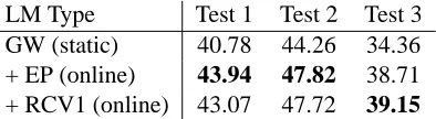
[image:9.612.139.233.58.154.2]LM Type Test 1 Test 2 Test 3 GW (static) 41.69 42.40 35.48 + RCV1 (online) 42.44 43.83 40.55 + EP (online) 42.80 43.94 38.82
Table 9: Test results for the RCV1 stream using the large background LM. Using stream data benefits translation.
based translation experiments using a large back-ground LM trained on a billionn-grams.
We used the same setup described in Section 5.1. However, instead of using only a subset of the GW corpus as one of our incoming streams, we trained a static LM using the full GW3 corpus of over three billion tokens and used it as a background LM. As then-gram statistics for this background LM show in Table 8, it contains far more data than each of the stream specific LMs (Table 1). We tested whether using streams atop this large background LM had a positive effect on translation for a given domain.
Baseline results for all test points using only the GW background LM are shown in the top row in Tables 9 and 10. We then interpolated the ORLMs with this LM. For each stream test point we interpo-lated with the big GW LM an online LM built with the most recent epoch’s data. Here we used sepa-rate models per stream so the RCV1 test points used the GW LM along with a RCV1 specific ORLM. We used the same mechanism to obtain the interpolation weights as described in Section 5.3 and minimised the perplexity of the static LM along with the stream specific ORLM. Interestingly, the tuned weights re-turned gave approximately a 50-50 weighting be-tween LMs and we found that simply using a 50-50 weighting for all test points resulted had no negative effect on BLEU. In the third row of the Tables 9 and 10 we show the results of interpolating the big
back-LM Type Test 1 Test 2 Test 3 GW (static) 40.78 44.26 34.36 + EP (online) 43.94 47.82 38.71 + RCV1 (online) 43.07 47.72 39.15
Table 10: EP test results using the background GW LM.
ground LM with ORLMs built using the approach described in Section 4.4. In this case all streams were combined into a single LM using a subsam-pling rate for higher ordern-grams. As before our sampling rate for the newswire streams was 30% chosen by the perplexity reduction weights.
The results show that even with a large amount of static data adding small amounts of stream spe-cific data relevant to a given test point has an im-pact on translation quality. Compared to only us-ing the large background model we obtain signifi-cantly better results when using a streaming ORLM to compliment it for all test domains. However the large amount of data available to the decoder in the background LM positively impacts translation performance compared to single-stream approaches (Tables 2 and 3). Further, when we combine the streams into a single LM using the subsampling ap-proach we get, on average, comparable scores for all test points. Thus we see that the patterns for multi-ple stream adaptation seen in previous sections hold in spite of big amounts of static data.
7 Conclusions and Future Work
We have shown how multiple streams can be effi-ciently incorporated into a translation system. Per-formance need not degrade on any of the streams. As well, these results can be additive. Even when using large amounts of additional background data, adding stream specific data continues to improve translation. Further, we achieve all results in bounded space. Future work includes investigating more sophisticated adaptation for multiple streams. We also plan to explore alternative ways of sampling the stream when incorporating data.
Acknowledgements
[image:9.612.86.289.201.258.2]pro-gram, DARPA Contract No. HR0011-06-C-0022 and by ESPRC Grant No. EP/I010858/1bb.
References
Thorsten Brants, Ashok C. Popat, Peng Xu, Franz J. Och, and Jeffrey Dean. 2007. Large language models in machine translation. In Proceedings of the 2007 Joint
Conference on Empirical Methods in Natural guage Processing and Computational Natural Lan-guage Learning (EMNLP-CoNLL), pages 858–867.
Amit Goyal, Hal Daum´e III, and Suresh Venkatasubra-manian. 2009. Streaming for large scale NLP: Lan-guage modeling. In North American Chapter of the
Association for Computational Linguistics (NAACL),
Boulder, CO.
David Graff, Junbo Kong, Ke Chen, and Kazuaki Maeda. 2007. English Gigaword Third Edition. Linguistic Data Consortium (LDC-2007T07).
Nathalie Japkowicz and Shaju Stephen. 2002. The class imbalance problem: A systematic study. Intell. Data
Anal., 6:429–449, October.
Philipp Koehn and Hieu Hoang. 2007. Factored transla-tion models. In Proceedings of the 2007 Joint
Confer-ence on Empirical Methods in Natural Language Pro-cessing and Computational Natural Language Learn-ing (EMNLP-CoNLL), pages 868–876.
Philipp Koehn and Josh Schroeder. 2007. Experiments in domain adaptation for statistical machine transla-tion. In Proceedings of the Second Workshop on
Sta-tistical Machine Translation, pages 224–227, Prague,
Czech Republic, June. Association for Computational Linguistics.
Philipp Koehn. 2003. Europarl: A multilingual corpus for evaluation of machine translation. Available at: http://www.statmt.org/europarl/. Abby Levenberg and Miles Osborne. 2009.
Stream-based randomised language models for SMT. In
Pro-ceedings of the Conference on Empirical Methods in Natural Language Processing (EMNLP).
Yishay Mansour, Mehryar Mohri, and Afshin Ros-tamizadeh. 2008. Domain adaptation with multiple sources. In NIPS, pages 1041–1048.
Kishore Papineni, Salim Roukos, Todd Ward, and Wei-Jing Zhu. 2001. Bleu: a method for automatic evalua-tion of machine translaevalua-tion. In ACL ’02: Proceedings
of the 40th Annual Meeting on Association for Compu-tational Linguistics, pages 311–318, Morristown, NJ,
USA. Association for Computational Linguistics. Tony Rose, Mark Stevenson, and Miles Whitehead.
2002. The reuters corpus volume 1 - from yester-days news to tomorrows language resources. In In
Proceedings of the Third International Conference on Language Resources and Evaluation, pages 29–31.
David Talbot and Thorsten Brants. 2008. Randomized language models via perfect hash functions. In
Pro-ceedings of ACL-08: HLT, pages 505–513, Columbus,
Ohio, June. Association for Computational Linguis-tics.
David Talbot and Miles Osborne. 2007. Smoothed Bloom filter language models: Tera-scale LMs on the cheap. In Proceedings of the 2007 Joint Conference
on Empirical Methods in Natural Language Process-ing and Computational Natural Language LearnProcess-ing (EMNLP-CoNLL), pages 468–476.
Hua Wu, Haifeng Wang, and Chengqing Zong. 2008. Domain adaptation for statistical machine translation with domain dictionary and monolingual corpora. In
Proceedings of the 22nd International Conference on Computational Linguistics (Coling 2008), pages 993–