A New Feature Selection Technique Combined with ELM Feature Space for Text Classification

(1)

D S Sharma, R Sangal and A K Singh. Proc. of the 13th Intl. Conference on Natural Language Processing, pages 285–292, Varanasi, India. December 2016. c2016 NLP Association of India (NLPAI)

A New Feature Selection Technique Combined with ELM Feature Space

for Text Classification

Rajendra Kumar Roul

Dept of Computer Science and Information System

BITS,Pilani-K.K.Birla Goa Campus Zuarinagar

Goa-403726

[email protected]

Pranav Rai

Dept of Electrical and Electronics Engineering BITS,Pilani-K.K.Birla Goa Campus

Zuarinagar Goa-403726

[email protected] Abstract

The aim of text classification is to classify the text documents into a set of pre-defined categories. But the complexity of natural languages, high dimensional feature space and low quality of feature selection be-come the main problem for text classifica-tion process. Hence, in order strengthen the classification technique, selection of important features, and consequently re-moving the unimportant ones is the need of the day. The Paper proposes an ap-proach called Commonality-Rarity Score Computation(CRSC)for selecting top fea-tures of a corpus and highlights the impor-tance of ML-ELM feature space in the do-main of text classification. Experimental results on two benchmark datasets signify the prominence of the proposed approach compared to other established approaches.

Keywords:Classification; ELM; Feature selec-tion; ML-ELM; Rarity

1 Introduction

With the increase in number of documents on the Web, it has become increasingly important to re-duce the noisy and redundant features which can reduce the training time and hence increase the performance of the classifier during text classifica-tion. Large number of features, produces feature vector with very high dimensionality and hence, different methods to reduce the dimension can be used such as Singular Value Decomposition (SVD) (Golub and Reinsch, 1970), Wavelet Anal-ysis (Lee and Yamamoto, ), Principle Component Analysis (PCA)(Bajwa et al., 2009) etc. The al-gorithms used for feature selection are broadly classified into three categories: filters, wrapper and embedded methods. Filter methods use the properties of the dataset to select the features

without using any specific algorithm (Kira and Rendell, 1992), and hence preferred over wrap-per methods. Most filter methods give a rank-ing of the best features rather than one srank-ingle set of best features. Wrapper methods use a pre-decided learning algorithm i.e. a classifier to eval-uate the features and hence computationally ex-pensive (Kohavi and John, 1997). Also, they have a higher possibility of overfitting than filter methods. Hence, large scale problems like text categorization mostly do not use wrapper meth-ods (Forman, 2003). Embedded methmeth-ods tend to combine the advantages of both the aforemen-tioned methods. The computational complexity of the embedded methods, thus, lies in between that of the filters and the wrappers. Ample re-search work has already been done in this do-main (Qiu et al., 2011)(Lee and Kim, 2015)(Meng et al., 2011)(Novoviˇcov´a et al., 2007)(Yang et al., 2011)(Aghdam et al., 2009)(Thangamani and Thangaraj, 2010)(Azam and Yao, 2012)(Liu et al., 2005).

Selection of a good classifier plays a vital role in the text classification process. Many of the tradi-tional classifiers have their own limitations while solving any complex problems. On the other hand, Extreme Learning Machine (ELM) is able to ap-proximate any complex non-linear mappings di-rectly from the training samples (Huang et al., 2006b). Hence, ELM has a better universal ap-proximation capability than conventional neural networks based classifiers. Also, quick learning speed, ability to manage huge volume of data, re-quirement of less human intervention, good gener-alization capability, easy implementation etc. are some of the salient features which make ELM more popular compared to other traditional classi-fiers. Recently developed Multilayer ELM which is based on the architecture of deep learning is an extension of ELM and have more than one hidden layer.

(2)

In this paper, we propose an approach for fea-ture selection called Commonality-Rarity Score Computation (CRSC) by means of three param-eters (Alpha (measures weighted commonality), Beta (measures extent of occurrence of a term) and Gamma (average weight of term per docu-ment)), computes the score of a term in order to rank them based on their relevance. The top m% features are selected for text classification. The proposed approach is compared with traditional feature selections techniques such as Chi-Square (Manning and Raghavan, 2008), Bi-normal sep-aration (BNS) (Forman, 2003), Information Gain (IG)(Yang and Pedersen, 1997) and GINI (Shang et al., 2007). Empirical results on 20-Newsgroups and Reuters datasets show the effectiveness of the proposed approach compared to other feature se-lection techniques.

The paper is outlined as follows: Section 2 dis-cussed the architecture of ELM, ML-ELM and ML-ELM extended feature space. The proposed approach is described in Section 3. Section 4 cov-ers the experimental work and finally, the paper is concluded in Section 5.

2 Background

2.1 ELM in Brief

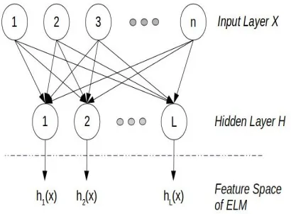
Given an input feature vectorx ofN documents andLhidden neurons, the output function of ELM for one node (Huang et al., 2006b) is

y(x) =h(x)β =

L X

i=1

βihi(x) (1)

Here,hi(x)←g(wi.xj+bi),∀j∈N,

wi ←input weight vector,

bi←ithhidden node biases,

β←the output weight vector between the hidden and output layer nodes.

The input feature vector and biases of the hidden layer nodes are selected randomly. The activation functiong(x) maps the input feature vector to an Ldimensional hidden layer space called ELM fea-ture space (Figure 2). The reduced form of equa-tion 1 whereY andHoutput and hidden layer ma-trix, respectively can be written as

Hβ=Y (2)

2.2 Brief on Multilayer ELM

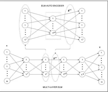
Multilayer ELM suggested by (Kasun et al., 2013) is based on the architecture of of deep learning and

[image:2.612.330.552.86.275.2]

is shown in the Figure 1. It combines bot ELM and ELM-autoencoder (ELM-AE) together, and hence contains all features of ELM.

Figure 1: Architecture of Multiayer ELM

The design and architecture of ELM-AE is same as ELM except few differences are exist between them such as

1. In ELM, input weights and biases of hid-den layer are randomly assigned where as in ELM-AE, both are orthogonal i.e.

wT ·w=I and bT ·b= 1

2. ELM is supervised in nature where the output is class labels. But ELM-AE is unsupervised in nature and the output is same as the input.

3. Computing β in ELM-AE is different then ELM and can be done using the following equations depending on the relationship be-tweennandL.

i. Compress representation(n > L):

β=

I C +H

T_H ₋1

HTX (3)

where, C is is scaling parameter used to adjusts the structural and experiential risk.

ii. Dimension of equal length(n=L):

β=H−1X (4)

iii. Sparse representation(n < L):

β =HT(I

C +HH

T₎−1_X ₍₅₎

(3)

According to (Huang et al., 2006a)(Huang et al., 2012), by increasing the number of nodes in the hidden layer compared to the input layer, the in-put feature vector become much simpler and thus linear separable in the extended space. Multilayer ELM uses the properties ofELM feature mapping and thus classify the features in a better manner which enhance its performance compared to other traditional classifiers.

The following equation is used to pass the data from one layer to another till it reaches the(n₋ 1)thhidden layer.

Hn=g((βn)THn-1) (6)

[image:3.612.89.294.310.461.2]

At the end, the final output matrix is generated by using the regularized least squares technique in or-der to calculate the results between the output and (n−1)thhidden layer.

Figure 2: ELM feature space

3 Proposed Approach

The aim of a good feature selection technique is to effectively distinguish between terms that are relevant and those that are not. For this purpose, the meaning of ‘relevance’ needs to be considered clearly. Some methods understand ‘relevance’ on the basis of the relation of the term to a particu-lar class. Other feature selection methods rely on probabilistic or statistical models to select the ap-propriate terms. For Commonality Rarity Score Computation (CRSC), a term is ‘relevant’ if it has the following attributes:

i. It does not appear very frequently in the cor-pus, as it would then be unsuitable as a dif-ferentiator between documents.

ii. It’s frequency in the corpus is not very low, as it would then be unsuitable to be used for grouping similar documents.

iii. In the documents in which the term appears, it should be reasonably frequent.

iv. It needs to be a good discriminator at the doc-ument level.

In order to apply these properties to a mathe-matical definition of relevance, we propose three parameters, whose combination would provide a score to each term. If the score of a term would be higher then its its relevance is higher. The param-eters mentioned above are alpha (α(t)), beta (β(t)) and gamma (γ(t)), each of which will be consid-ered in detail in the next section.

3.1 Alpha

The parameter alpha (α(t)), is a mathematical rep-resentation of the weighted commonality of the termtand is defined as

α(t) = ( 1

idf ∗y) + (idf ∗(1−y)) (7)

where,

y= a N and

idf =

N X

t

idf(t) N

Here, ‘a’ represents the number of documents with the termtandN represents total number of documents in the corpus. The IDF of a term indi-cates the rarity of the term in the corpus.

IDF(t) = 1 +log10(N

a)

The average IDF (idf) denotes the average rarity of the corpus.

(4)

the value ofα(t)iff the termtis rare and the aver-age rarity of the terms in the corpus is high. Thus, the equation forα(t) provides a method to com-pute a commonality-rarity of a term in the corpus. Sinceidf of a term is always greater than 1, there-fore, idf will be more than 1. Also, if a term is very rare, it’s (1-y) value will be high which makes the value ofα(t)for that term as high. Hence, rare terms tend to have higher values for α(t). This feature is used to filter the unimportant terms, as explained in section 3.4.

3.2 Beta

The parameter beta(β(t)), is a mathematical rep-resentation of the frequency of appearance of the termtin the documents and can be given by

β(t) =y1(t) +y22(t) +y33(t) +...

where

yi(t) = ai

N (8)

where ai ← number of documents where

fre-quency oft_≥i. The termβ(t)therefore provides information regarding the prevalence of the termt in the corpus by considering the fraction of doc-uments containing the termtand also taking into account the frequency of appearance of the term in each document. Terms which appear frequently in several documents will have a higher beta value. Also, the contribution ofyitoβ(t)decreases with

increasing value of i. Therefore, very high fre-quency of occurrence of a term t in a particular document does not significantly increase itsβ(t). This is done mathematically by giving eachyi as

an exponenti.

3.3 Gamma

Gamma (γ(t)) is obtained by summing over all documentsd in the corpus of γ(t, d) and can be written as

γ(t, d) = TF(t, d)

maximum TF ind (9)

γ(t, d) gives an indication of the relative weight of the termtin the documentd, by comparing the frequency of the termt to the highest frequency term ind. γ(t)quantitatively denotes the average weighted frequency of the term per document in the corpus.

3.4 Score

Finally, using the above three parameters, a total score is assigned to each term in the corpus as an indication of its relevance. The score of a termtis given by

score(t) =β(t)_∗min(γ(t),1/γ(t))₋α(t) (10)

A higher value of score(t) indicates a higher relevance of the term t to the corpus. As elab-orated previously, β(t) indicates the overall frequency of a term in the corpus, and the term γ(t) indicates the average frequency of the term in each document in the corpus. A high value for β(t) indicates that very frequently t is present in most of the documents, whereas a high value for γ(t) suggests that the term t is frequent in those documents where it is present, and therefore a good discriminator for the same. For a term t to be a good differentiator among documents, not only must it be frequent in the corpus, but it must also be important for differentiating between documents. For this, γ(t) should necessarily not be very low for a term, which is to be selected as part of the reduced feature space to classify the documents. However, a direct product of β(t) andγ(t) can result in common terms that appear in almost all documents given very high scores, despite them not being relevant per our earlier definition. In order to eliminate such terms, we instead use a product ofβ(t)and the minimum of γ(t) and 1/γ(t). With this product, terms which are very frequent, and as a result have a high value for β(t), will result in the β(t)value being divided by their equally largeγ(t)value, reducing their score, and preventing such terms being considered as important. The term α(t), which takes high values for rare terms, is subtracted from the previous product to produce the score. This eliminates those terms that are very rare from being considered as important.

(5)

pus level.

3.5 Algorithm

Proposed approach ofCRSCis discussed below. Step 1. Documents pre-processing and vector

repre-sentation:

The documents d = _{d1, d2, ..., dm} of all

classes of a corpus are collected and pre-processed by using a pre-processing algo-rithm. Then, all the documents are converted into vectors using the formal Vector Space Model (VSM)(Salton et al., 1975).

Step 2. Formation of clusters:

Traditional k-means clustering algorithm (Hartigan and Wong, 1979) is run on the cor-pus to generates k term-document clusters, tdi, i= 1, ..., k.

Step 3. Important features selection:

Now, for each term t ∈ tdi, α(t), β(t) and

γ(t) are calculated and then the total score using equation 10 is computed.

Step 4. Training ML-ELM and other conventional classifiers:

Based on the total score, all the terms of a cluster are ranked and top m% terms from each cluster are selected which constitute the training feature vector.

4 Experimental Analysis

20-Newsgroups1 _{and Reuters}2 _{datasets are used} for experimental purpose. The classifiers which are used for comparison purpose are Support Vec-tor Machine (LinearSVC), Decision Tree (DT), SVM linear kernel (LinearSVM), Gaussian Naive Bayes (GNB), Random Forest (RF), Nearest Cen-troid (NC), Adaboost, Multinomial Naive-Bayes (M-NB) and ELM. In all the tables bold indicates the highest F-measure obtained byCRSCusing the corresponding classifier. The algorithm was tested on hidden layer nodes of different size both for ELM and ML-ELM and the best results are ob-tained when the number of nodes of hidden layer are more than the nodes in the input layer. In the k-means clustering,k(the number of clusters) was set as 8 (decided empirically) for both the datasets. The following parameters are used to measure the performance.

1_{http://qwone.com/}_∼_{jason/20Newsgroups/}

2_{www.daviddlewis.com/resources/testcollections/reuters/}

Precision (P):

P= (relevantdocuments)∩(retrieveddocuments) retrieveddocuments

Recall (R):

R= (relevantdocuments)∩(retrieveddocuments) relevantdocuments

F-Measure (F):It combines both precision and re-call and can be defined as follows:

F= 2 (P×R) (P+R)

4.1 20-Newsgroups Dataset

20-Newsgroups is a very popular machine learn-ing dataset generally used for text classification and having 7 different categories. For experimen-tal purpose, approximately 11300 documents are used for training and 7500 for testing. The results can be summarized as follows:

- top 1% features: CRSCusing ML-ELM and Multinomial naive-bayes has obtained the best results. Classifier wise, ML-ELM gen-erates the maximum average F-measure for CRSC(Table 1).

- top 5% features: ML-ELM and LinearSVM generate the best results. Classifier wise, maximum average F-measure is obtained us-ing ML-ELM (Table 2).

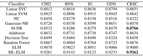
[image:5.612.317.552.632.725.2]

- top 10% features: CRSC has obtained best results using ML-ELM and Random Forest. Classifier wise CRSC obtained the highest average F-measure of 0.9602 using ML-ELM (Table 3).

Table 1: F-measure on top 1% features (20-NG)

Classifier CHI2 BNS IG GINI CRSC Linear SVC 0.8812 0.8616 0.8636 0.8794 0.8651 Linear SVM 0.8925 0.8896 0.8915 0.8945 0.8842 NC 0.8458 0.8278 0.8338 0.8516 0.8222 Gaussian-NB 0.8726 0.8530 0.8599 0.8651 0.8078 M-NB 0.8532 0.8286 0.8279 0.8479 0.8766

Adaboost 0.8632 0.8731 0.8738 0.8747 0.8634 Decision Tree 0.8499 0.8484 0.8490 0.8324 0.8458 Random Forest 0.8867 0.8660 0.8764 0.8723 0.8676 ELM 0.9070 0.9023 0.8951 0.9066 0.9080 ML-ELM 0.9261 0.9143 0.9123 0.9233 0.9262

(6)

Classifier CHI2 BNS IG GINI CRSC LinearSVC 0.9246 0.9187 0.9181 0.9315 0.9245 LinearSVM 0.9337 0.9241 0.9279 0.9337 0.9359

NC 0.8895 0.8756 0.8848 0.8859 0.8690 Gaussian-NB 0.9257 0.8787 0.8925 0.9187 0.8515 M-NB 0.9212 0.8914 0.9060 0.9151 0.8819 Adaboost 0.8876 0.8736 0.8526 0.8613 0.8682 Decision Tree 0.8499 0.8527 0.8481 0.8476 0.8461 Random Forest 0.8942 0.8702 0.8922 0.8842 0.8771 ELM 0.9287 0.9288 0.9366 0.9358 0.9374 ML-ELM 0.9345 0.9432 0.9378 0.0.9452 0.9450

Classifier CHI2 BNS IG GINI CRSC LinearSVC 0.9374 0.9273 0.9368 0.9437 0.9392 LinearSVM 0.9428 0.9355 0.9364 0.9465 0.9353 NC 0.8947 0.8858 0.8886 0.8951 0.8858 Gaussian-NB 0.9297 0.9011 0.9235 0.9293 0.8613 M-NB 0.9282 0.9134 0.9227 0.9273 0.9093 Adaboost 0.8727 0.8526 0.8534 0.8625 0.8568 Decision Tree 0.8537 0.8392 0.8560 0.8491 0.8464 Random Forest 0.8829 0.8825 0.8740 0.8827 0.8857

ELM 0.9467 0.9388 0.9257 0.9484 0.9596 ML-ELM 0.9515 0.9422 0.9367 0.9521 0.9602

4.2 Reuters Dataset

Reuters is a widely used dataset, predominantly utilized for text mining. It has 5485 training doc-uments and 2189 testing docdoc-uments classified into 8 classes, where all class documents are consid-ered for evaluation. Out of 17512 features from all documents, 12345 features are considered for training. The results are summarized as follows:

- top 1% features: CRSC using Adaboost has obtained the best results. Classifier wise, Lin-earSVM generates the maximum average F-measure forCRSC(Table 4).

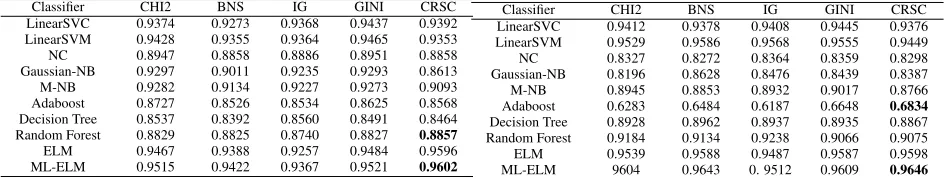
- top 5% features: Adaboost and ML-ELM generate the best results. Classifier wise, maximum average F-measure is obtained us-ing ML-ELM (Table 5).

[image:6.612.80.552.63.152.2]

- top 10% features: CRSC has obtained the best results using ML-ELM and Adaboost. Classifier wise CRSC obtained the highest average F-measure of 0.9598 using ML-ELM (Table 6).

4.3 Discussion

Figure 3 - 5 show the performance comparison of different classifiers on top m% features using CRSCfeature selection technique. Comparison of ELM with other traditional classifiers on CRSC are shown in Table 7. It is evident from all the re-sults that ML-ELM outperforms other well known classifiers.

Table 4: F-measure on top 1% features (Reuters)

Classifier CHI2 BNS IG GINI CRSC LinearSVC 0.9236 0.9137 0.9196 0.9297 0.8954 LinearSVM 0.9424 0.9391 0.9414 0.9495 0.9196 NC 0.8238 0.8242 0.8215 0.8283 0.8045 Gaussian-NB 0.8544 0.8453 0.8434 0.8434 0.8414 M-NB 0.8620 0.8318 0.8483 0.8503 0.8352 Adaboost 0.6300 0.6405 0.6435 0.7625 0.7798

[image:6.612.80.553.187.276.2]

Decision Tree 0.8816 0.8785 0.8804 0.8858 0.8548 Random Forest 0.9123 0.9195 0.9136 0.9124 0.8995 ELM 0.9444 0.9467 0.9468 0.9579 0.9161 ML-ELM 0.9531 0.9484 0.9522 0.9590 0.9178

[image:6.612.315.552.313.404.2]

Decision Tree 0.8928 0.8962 0.8937 0.8935 0.8867 Random Forest 0.9184 0.9134 0.9238 0.9066 0.9075 ELM 0.9539 0.9588 0.9487 0.9587 0.9598 ML-ELM 9604 0.9643 0. 9512 0.9609 0.9646

[image:6.612.313.558.439.534.2]

Decision Tree 0.8955 0.8885 0.8968 0.8894 0.8965 Random Forest 0.9090 0.9069 0.9090 0.9098 0.9007 ELM 0.9472 0.9489 0.9477 0.9432 0.9588 ML-ELM 0.9566 0.9654 0.9645 0.9678 0.9598

Table 7: F-measure comparisons onCRSC

Classifier _1%20- NG (F-Measure-%)_5% _10% _1%Reuters (F-Measure-%)_5% _10%

LinearSVC 86.51 92.45 93.92 89.54 93.76 94.47 Linear SVM 88.42 93.59 93.53 91.96 94.49 95.78 NC 82.22 86.90 88.58 80.45 82.98 83.51 G-NB 80.78 85.15 86.13 84.14 83.87 78.14 M-NB 87.66 88.19 90.93 83.52 87.66 87.69 Adaboost 86.34 86.82 85.68 77.98 68.34 64.32 DT 84.58 84.61 84.64 85.48 88.67 89.65 RF 86.76 87.71 88.57 89.95 90.75 90.07 ELM 90.80 93.74 95.96 91.61 95.98 95.88 ML-ELM 92.62 94.5 96.02 91.78 96.46 95.98

5 Conclusion

(7)

[image:7.612.97.296.36.184.2] [image:7.612.95.295.242.390.2]

Figure 3: F-measure ofCRSCfor top-1%

techniques. The results obtained by ML-ELM which uses the ELM feature mapping technique by which makes the features linearly separable in the extended space, dominated all other state-of-the-art classifiers.

References

[Aghdam et al.2009] Mehdi Hosseinzadeh Aghdam, Nasser Ghasem-Aghaee, and Mohammad Ehsan Basiri. 2009. Text feature selection using ant colony optimization. Expert systems with applica-tions, 36(3):6843–6853.

[Azam and Yao2012] Nouman Azam and JingTao Yao. 2012. Comparison of term frequency and docu-ment frequency based feature selection metrics in text categorization. Expert Systems with Applica-tions, 39(5):4760–4768.

[image:7.612.81.299.448.592.2]

[Bajwa et al.2009] Imran S Bajwa, M Naweed, M Nadim Asif, and S Irfan Hyder. 2009. Feature based image classification by using principal com-ponent analysis. ICGST Int. J. Graph. Vis. Image Process. GVIP, 9:11–17.

[Forman2003] George Forman. 2003. An extensive empirical study of feature selection metrics for text classification. The Journal of machine learning re-search, 3:1289–1305.

[Golub and Reinsch1970] Gene H Golub and Christian Reinsch. 1970. Singular value decomposition and least squares solutions. Numerische mathematik, 14(5):403–420.

[Hartigan and Wong1979] John A Hartigan and Manchek A Wong. 1979. Algorithm as 136: A k-means clustering algorithm. Journal of the Royal Statistical Society. Series C (Applied Statistics), 28(1):100–108.

[Huang et al.2006a] Guang-Bin Huang, Lei Chen, Chee Kheong Siew, et al. 2006a. Universal approximation using incremental constructive feed-forward networks with random hidden nodes.IEEE Transactions on Neural Networks, 17(4):879–892.

[Huang et al.2006b] Guang-Bin Huang, Qin-Yu Zhu, and Chee-Kheong Siew. 2006b. Extreme learning machine: theory and applications.Neurocomputing, 70(1):489–501.

[Huang et al.2012] Guang-Bin Huang, Hongming Zhou, Xiaojian Ding, and Rui Zhang. 2012. Extreme learning machine for regression and multiclass classification.IEEE Transactions on Sys-tems, Man, and Cybernetics, Part B (Cybernetics), 42(2):513–529.

[Kasun et al.2013] Liyanaarachchi Leka-malage Chamara Kasun, Hongming Zhou, Guang-Bin Huang, and Chi Man Vong. 2013. Representational learning with extreme learning machine for big data. IEEE Intelligent Systems, 28(6):31–34.

[Kira and Rendell1992] Kenji Kira and Larry A Ren-dell. 1992. The feature selection problem: Tradi-tional methods and a new algorithm. InAAAI, vol-ume 2, pages 129–134.

(8)

[Kohavi and John1997] Ron Kohavi and George H John. 1997. Wrappers for feature subset selection. Artificial intelligence, 97(1):273–324.

[Lee and Kim2015] Jaesung Lee and Dae-Won Kim. 2015. Mutual information-based multi-label feature selection using interaction information. Expert Sys-tems with Applications, 42(4):2013–2025.

[Lee and Yamamoto] Daniel TL Lee and Akio Ya-mamoto. Wavelet analysis: theory and applications. Hewlett Packard journal, 45:44–44.

[Liu et al.2005] Luying Liu, Jianchu Kang, Jing Yu, and Zhongliang Wang. 2005. A comparative study on unsupervised feature selection methods for text clustering. In Natural Language Processing and Knowledge Engineering, 2005. IEEE NLP-KE’05. Proceedings of 2005 IEEE International Conference on, pages 597–601. IEEE.

[Manning and Raghavan2008] Christopher Manning and Prabhakar Raghavan. 2008. Introduction to information retrieval.

[Meng et al.2011] Jiana Meng, Hongfei Lin, and Yuhai Yu. 2011. A two-stage feature selection method for text categorization. Computers & Mathematics with Applications, 62(7):2793–2800.

[Novoviˇcov´a et al.2007] Jana Novoviˇcov´a, Petr Somol, Michal Haindl, and Pavel Pudil, 2007. Progress in Pattern Recognition, Image Analysis and Ap-plications: 12th Iberoamericann Congress on Pat-tern Recognition, CIARP 2007, Valparaiso, Chile, November 13-16, 2007. Proceedings, chapter Con-ditional Mutual Information Based Feature

Se-lection for Classification Task, pages 417–426. Springer Berlin Heidelberg, Berlin, Heidelberg.

[Qiu et al.2011] Xipeng Qiu, Jinlong Zhou, and Xu-anjing Huang. 2011. An effective feature selec-tion method for text categorizaselec-tion. InAdvances in Knowledge Discovery and Data Mining, pages 50– 61. Springer.

[Salton et al.1975] Gerard Salton, Anita Wong, and Chung-Shu Yang. 1975. A vector space model for automatic indexing. Communications of the ACM, 18(11):613–620.

[Shang et al.2007] Wenqian Shang, Houkuan Huang, Haibin Zhu, Yongmin Lin, Youli Qu, and Zhihai Wang. 2007. A novel feature selection algorithm for text categorization. Expert Systems with Appli-cations, 33(1):1–5.

[Thangamani and Thangaraj2010] M Thangamani and P Thangaraj. 2010. Integrated clustering and fea-ture selection scheme for text documents 1.

[Yang and Pedersen1997] Yiming Yang and Jan O Ped-ersen. 1997. A comparative study on feature se-lection in text categorization. InICML, volume 97, pages 412–420.

[Yang et al.2011] Jieming Yang, Yuanning Liu, Zhen Liu, Xiaodong Zhu, and Xiaoxu Zhang. 2011. A new feature selection algorithm based on binomial hypothesis testing for spam filtering. Knowledge-Based Systems, 24(6):904–914.