Simulating the future wind energy resource of Ireland using the COSMO CLM model

RESEARCH ARTICLE

Simulating the future wind energy resource of Ireland

using the COSMO-CLM model

Paul Nolan, Peter Lynch and Conor Sweeney

Meteorology and Climate Department, University College Dublin, Dublin, Ireland

ABSTRACT

We consider the impact of climate change on the wind energy resource of Ireland using an ensemble of regional climate model (RCM) simulations. The RCM used in this work is the Consortium for Small-scale Modelling–climate limited-area modelling (COSMO-CLM) model.

The COSMO-CLM model was evaluated by performing simulations of the past Irish climate, driven by European Centre for Medium-Range Weather Forecasts ERA-40 data, and comparing the output with observations. For the investigation of the influence of the future climate under different climate scenarios, the Max Planck Institute’s global climate model, ECHAM5, was used to drive the COSMO-CLM model. Simulations are run for a control period 1961–2000 and future period 2021–2060. To add to the number of ensemble members, the control and future simulations were driven by different realizations of the ECHAM5 data. The future climate was simulated using the Intergovernmental Panel on Climate Change emission scenarios, A1B and B1.

The research was undertaken to consolidate, and as a continuation of, similar research using the Rossby Centre’s RCA3 RCM to investigate the effects of climate change on the future wind energy resource of Ireland. The COSMO-CLM projections outlined in this study agree with the RCA3 projections, with both showing substantial increases in 60 m wind speed over Ireland during winter and decreases during summer. The projected changes of both studies were found to be statistically significant over most of Ireland. The agreement of the COSMO-CLM and RCA3 simulation results increases our confidence in the robustness of the projections. Copyright © 2012 John Wiley & Sons, Ltd.

KEYWORDS

climate change; wind energy; Ireland; regional climate model; ensemble

Correspondence

Paul Nolan, Meteorology and Climate Department, University College Dublin, Dublin, Ireland. E-mail: [email protected]

Received 12 October 2011; Revised 14 August 2012; Accepted 14 August 2012

1. INTRODUCTION

The analysis presented in this paper was undertaken to investigate whether global climate change will lead to changes in the wind climatology of Ireland. There is considerable interest in renewable energy resources as a means of reducing carbon dioxide emissions to minimize climate change. From a climate perspective, Ireland is ideally located to exploit the natural energy associated with the wind: mean annual speeds are typically in the range 6–8.5 m s1at 60 m level over land, values that are sufficient to sustain commercial enterprises with current wind turbine technology.

The wind energy potential of the past Irish climate has been well documented.1–3However, climate change may alter the wind patterns in the future; a reduction in speeds may reduce the commercial returns or pose problems for the continuity of supply; an increase in the frequency of severe winds (e.g. gale/storm gusts) may similarly impact on supply continuity. Conversely, an increase in the mean wind speed may have a positive effect on the available power supply.

The impact of greenhouse gases on climate change can be simulated using global climate models (GCMs). However, long climate simulations using coupled atmosphere–ocean general circulation models are currently feasible only with horizontal resolutions of 50 km or greater. Since wind speed and direction are closely correlated to the local topography, this is inadequate for the simulation of the detail and pattern of climate change and its effects on the wind resource. The regional climate model (RCM) method dynamically downscales the coarse information provided by the

global models and provides high resolution information on a sub-domain covering Ireland. The computational cost of running the RCM, for a given resolution, is considerably less than a global model. The reader is referred to the RCM overviews by Dickinson,4 Giorgi5,6 and Christensen et al.7 A disadvantage of this downscaling approach is the fact that the lateral boundary conditions required to drive the RCM add a factor of uncertainty absent in global models, because they pose a constraint to the dynamics that interferes with the solution.8–10 Giorgi and Mearns11 present an overview of several additional issues regarding regional climate modelling. It is noted by Qianet al.12that models with relatively good skill at forecasting up to a few days can exhibit large biases for long-term climate simulations. To overcome this problem, studies such as by Qianet al.12have suggested a reinitialized approach, where the long-term continuous integration is split into smaller ones. This method is rarely used in regional climate simulations. Lo et al.13 highlighted three reasons for this: ‘First, the re-initialization approach may not be easily portable as additional scripts are needed to handle the re-initialization process. Second, the long spin-up time of RCMs constrains the re-initialization frequency. Third, there may be discontinuity points when results are applied to a transport model. Typically it takes a few hours to a few days for the driving ICs and LBCs to reach dynamical equilibrium with the internal model physics in RCMs. On the other hand, for the soil components, the spin-up time may take a few weeks to a year.14’Despite the problems outlined earlier, it was decided that in order to obtain future climate projections at high spatial resolution, the RCM approach is the best method available and should therefore be used for the current study. The RCM used in this work is the CLM Community’s Consortium for Small-scale Modelling– climate limited-area modelling (COSMO-CLM) model.15

The current research was undertaken to consolidate, and as a continuation of, similar research16,17using the Rossby Centre’s RCA3 RCM18,19to investigate the future wind energy resource of Ireland. The RCA3 model was driven at the lateral boundaries by ECHAM GCM data.20 The future climate was simulated using the four Intergovernmental Panel on Climate Change (IPCC) emission scenarios A1B, A2, B1 and B2.21Simulations were run for control period 1961–2000 and future period 2021–2060. Results for the RCA3 simulations showed a substantial overall increase in the energy content of the wind for the future winter months and a decrease during the summer months. The projected changes for summer and winter were found to be statistically significant over most of Ireland. However, the uncertainty of these projections was found to be high since the climate change signal was of similar magnitude to the variability of the evaluation and control simulations. The current research aims to address this uncertainty by employing an ensemble of RCM simulations to study climate change.

The COSMO-CLM projections outlined in the current study agree with the RCA3 projections16in the sense that they show significant increases in the future wind energy resource over Ireland during winter and decreases during summer. The agreement of the COSMO-CLM and RCA3 projections increase our confidence in the robustness of the future projec-tions. Furthermore, the current research allows us to address the issue of RCM uncertainty by employing different versions of COSMO-CLM to simulate the climate. To address the issue of inherent climate variability, the control and future simu-lations were repeated, using different realizations of the ECHAM5 data to drive the RCMs. Climate variability was then assessed by comparing the climate change signals with the variability of the control simulations. In addition, the COSMO-CLM model was run at a higher resolution than the RCA3 model, thus allowing us to better assess the local effects of climate change on the wind energy resource.

A possible explanation for the inter-annual variability increase in wind speed noted by Nolanet al.16and the present study may be due to a future change in cyclone activity. Most GCMs summarized in IPCC AR422(chapter 10) produce fewer weak but more intense mid-latitude cyclones in the latter part of the 21st century. The increase in intense cyclones over the North Atlantic is found to occur particularly during winter. This projected change in cyclone activity is consistent with the wind speed projections presented in the present study and by Nolanet al.16of an increase during winter and a decrease during summer. A plausible explanation put forward for the projected changes in cyclone activity23 is that a decreased meridional temperature gradient and the associated reduced baroclinicity in the future climate could be responsible for the decrease of the total number of extratropical cyclones.24 The higher moisture supply due to a generally higher sea surface temperature and the related increase in latent heatfluxes could trigger strong intensity cyclones.25

2. OBJECTIVES

The main objective of the research is to evaluate future wind energy resources by simulating the wind climatology of Ireland at high resolution using the method of regional climate modelling. To achieve this, wefirst evaluate the ability of the RCM to accurately simulate the wind climatology. The RCM is evaluated by performing simulations of the past Irish climate and comparing the output with observational data. We then simulate the future wind climate for different greenhouse gas emission scenarios and determine if future climate projections of the RCM show substantial changes when compared with the past and whether the changes are significant. To address the issue of RCM uncertainty, different versions of COSMO-CLM are employed to simulate the climate. To address the issue of inherent climate variability, the control and future simulations are repeated, using different realizations of the ECHAM5 data to drive the RCMs.

3. MODELS AND METHODS

3.1. The COSMO-CLM regional climate model

The COSMO-CLM regional climate model15is the COSMO weather forecasting model in climate mode. It is applied and further developed by members of the CLM Community (www.clm-community.eu). The COSMO model (www. cosmo-model.org) is the non-hydrostatic operational weather prediction model used by the German Weather Service (DWD). A detailed description of the COSMO model is given by Doms and Schattler31and Steppeleret al.32The Irish climate was simulated using versions COSMO-CLM 3.2 and 4.0 at 0.0625(~ 7 km) resolution on a rotated grid. The grid width is the same in the latitudinal and longitudinal direction. The model domain has 9094 grid points and, in the vertical, there are 32 unequally spaced levels. A 2 year spin-up period was included for all simulations. The windfields were output at 1 hour intervals. The model domain is shown in Figure 1. The COSMO-CLM 3.2 model was integrated with a time step of 40 s using a three-time level leapfrog scheme with time-split treatment of acoustic and gravity waves. The COSMO-CLM 4.0 model was integrated with a time step of 40 s using a Runge–Kutta time integration scheme. There are also several differences between the model versions 3.2 and 4.0. In particular, the cloud and precipitation physics have been ex-panded including now the formation of cloud ice and the prognostic treatment of the precipitation components, rain and snow. The external data set prescribing soil types and land use characteristics has also slightly changed. For exam-ple, the model is now able to distinguish between evergreen and deciduous forest and includes effects of subscale var-iation of orography in some parameterizations.33

Figure 1.The CLM 7 km resolution model domain. Locations referred to throughout the paper are numbered as follows: 1 Belmullet, 2 Claremorris, 3 Shannon Airport, 4 Valentia Observatory, 5 Cork Airport, 6 Mullingar, 7 Dublin Airport, 8 Casement Aerodrome, 9

The COSMO-CLM 7 km simulations of the current study were driven at the lateral boundaries by CLM consortial sim-ulation data at 18 km resolution.34The CLM consortial simulations were performed using the COSMO-CLM 3.2 model. The boundary information is assigned at the lateral boundaries and at the upper boundary and relaxed towards the model domain using the relaxation technique by Davies and Turner.35For the present study, the width of the lateral boundary relaxation zone is set as eight grid boxes (~56 km) for the COSMO-CLM 3.2 simulations and 50 km for the COSMO-CLM 4.0 simulations.

Henceforth, the COSMO-CLM model will be referred to as the CLM model with versions 3.2 and 4.0 referred to as CLM3 and CLM4, respectively.

The CLM3 18 km consortial wind speeds were shown to exhibit large-scale positive biases with a peak of up to 2 m s1 in Eastern Europe and values of approximately 1 m s1over Ireland.34A preliminary investigation of the CLM3 7 km sim-ulation of the current study also showed an overestimation of wind speeds. After consultation with the CLM community, it was decided that a plausible explanation for this positive bias was that the model surface drag was too low causing an underestimation of the cross-isobarflow in the planetary boundary layer. It was therefore decided to increase the surface drag of the CLM4 simulations presented in this study. This was achieved by including the sub-grid scale orographic scheme of Lott and Miller36in the CLM4 simulations.

3.2. CLM evaluation simulations

The CLM models were evaluated by performing simulations of the past Irish climate (1979–2000) and comparing the out-put with observations. The 2 year spin-up period 1979–1980 is disregarded. Thus, the evaluation period of the current study is the 20 year period 1981–2000. The European Centre for Medium-Range Weather Forecasts ERA-40 global re-analysis data37were used to drive the CLM3 18 km resolution model consortial simulations34and these in turn were used to drive the following CLM 7 km resolution simulations:

• CLM3 ERA40 evaluation simulation 1981–2000 (denoted CLM3-ERA) • CLM4 ERA40 evaluation simulation 1981–2000 (denoted CLM4-ERA)

The CLM3 18 km consortial simulations have been evaluated by Hollweget al.34Note that the ERA-40 data are based on the assimilation of actual observations over the integration period. It follows that the CLM-ERA wind data are a measure of the‘true’windfield at the analysis scale.

3.3. The CLM control and future climate simulations

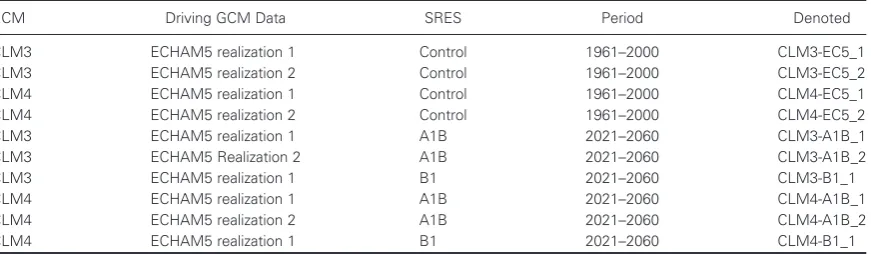
For the investigation of the influence of the future climate under different climate scenarios, the Max Planck Institute’s ECHAM5 GCM20 data were used to drive the CLM3 18 km simulations.34 The control and future simulations were repeated, using different realizations of the ECHAM5 data. The greenhouse gas emission scenarios were taken from those developed under the auspices of the IPCC Special Report on Emission Scenarios (SRES).21The CLM3 18 km simulations outlined by Hollweget al.34were used to drive the CLM 7 km resolution simulations presented in this study. Table I outlines the CLM 7 km resolution control and future simulations.

Table I. The COSMO-CLM 7 km control and future simulations.

RCM Driving GCM Data SRES Period Denoted

CLM3 ECHAM5 realization 1 Control 1961_–2000 CLM3-EC5_1

CLM3 ECHAM5 realization 2 Control 1961–2000 CLM3-EC5_2

CLM4 ECHAM5 realization 1 Control 1961–2000 CLM4-EC5_1

CLM4 ECHAM5 realization 2 Control 1961_–2000 CLM4-EC5_2

CLM3 ECHAM5 realization 1 A1B 2021_–2060 CLM3-A1B_1

CLM3 ECHAM5 Realization 2 A1B 2021–2060 CLM3-A1B_2

CLM3 ECHAM5 realization 1 B1 2021–2060 CLM3-B1_1

CLM4 ECHAM5 realization 1 A1B 2021_–2060 CLM4-A1B_1

CLM4 ECHAM5 realization 2 A1B 2021_–2060 CLM4-A1B_2

CLM4 ECHAM5 realization 1 B1 2021–2060 CLM4-B1_1

3.3.1. Realizations of the ECHAM5 simulations

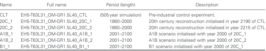
Table II gives an overview of the ECHAM5/MPIOM AR4 experiments38related to the regional projections outlined in Table I. All global experiments are started from model states obtained in a 505 year long integration of the coupled global model with pre-industrial conditions.34In that‘control’experiment (CTL), the concentrations of well-mixed greenhouse gases have been specified at the observed levels of 1860 and sulfate aerosols are not included. This reconstruction of a non-drifting climate is representative for the middle of the 19th century and provides the initialfields for the 20th century ECHAM5 global simulations with anthropogenic greenhouse and sulfate forcing. Fields from different years of CTL are used to initialise the different ECHAM5 realizations. The state of each ECHAM5 global ensemble realization at the end of year 2000 is used to initialise the ECHAM5 SRES climate projections. For further details of the outline of the ECHAM5/MPIOM experiments, refer to the document.38It should be noted that because of limited computation resources for the present study, a subset of the available ECHAM5/MPIOM experiments were downscaled. Furthermore, the‘B1_2’ experiment had to be abandoned as not all the boundary data were available.

3.4. Strategy for quality control

The quality control of the CLM simulations is based on both the comparison of the simulation results with observations and the comparison of the regional simulations with each other (Figure 2).

3.4.1. Comparisons of the CLM simulations

Test 1, the model evaluation, forms the basis of the quality control of the CLM model. In principle, the regional simulation CLM-ERA should provide the best possible representation of climate within the simulated domain. Therefore, this simulation serves as a reference run for all further model simulations. The quantitative comparison of this run with observations determines the quality of the CLM model. The difference between the output of the CLM3 and CLM4 simulations is also analysed.

The observed winds at Irish synoptic stations are measured at 10 m height. Thus, when comparing model output with obser-vations, the evaluations of test 1 focus on wind data at 10 m height. When comparing the model output with observed station

Table II. ECHAM5/MPIOM IPCC AR4 forcing for CLM.

Name Full name Period (length) Description

CLT EH5-T63L31_OM-GR1.5L40_CTL (505 year simulation) Pre-industrial control experiment.

20C_1 EH5-T63L31_OM-GR1.5L40_20C_1 1860–2000 20th century reconstruction initialised in year 2190 of CTL 20C_2 EH5-T63L31_OM-GR1.5L40_20C_2 1860–2000 20th century reconstruction initialised in year 2215 of CTL A1B_1 EH5-T63L31_OM-GR1.5L40_A1B_1 2001_–2100 A1B scenario initialised with year 2000 of 20C_1 A1B_2 EH5-T63L31_OM-GR1.5L40_A1B_2 2001_–2100 A1B scenario initialised with year 2000 of 20C_2 B1_1 EH5-T63L31_OM-GR1.5L40_B1_1 2001–2100 B1 scenario initialised with year 2000 of 20C_1

data, the model data were bilinearly interpolated onto the latitude–longitude station location. Figure 1 shows the locations of the synoptic stations referred to throughout this paper. The observed wind data for Rosslare station was limited to the 16 year period 1981–1996. The observed wind speeds are calculated each hour using the mean value in the preceding 10 min.

Since the CLM3 18 km simulations have previously been evaluated,34this study will primarily focus on the evaluation of the CLM 7 km simulations. The CLM3 18 km evaluation showed a positive bias in the mean 10 m wind speed of between 0 and 1 m s1over most of Ireland.

Test 2 investigates the quality of the control 7 km resolution simulations. The ECHAM5 climate simulations are uncon-strained by observations but nevertheless the downscaled CLM-ECHAM simulations should produce a windfield climatol-ogy that is close to the observed climate and the CLM-ERA simulations. The differences to the evaluation run CLM-ERA demonstrate the influence of the global climate simulations on the regional climate reconstruction. Furthermore, the com-parison captures the internal climate variability on the considered time scale. Test 2 focuses on wind data at 10 m height. Test 3 investigates the regional climate change signal of the 7 km resolution simulations. This comparison, along with tests 4 and 5 indicate the expected climate change signal and the potential uncertainty of the detected changes due to the internal variability of the climate system.

Test 4 compares the CLM-EC5 control 7 km resolution simulations. The magnitude of variability of this test is compared with the magnitude of the climate change signal of test 3 to determine if a level of confidence can be assigned to the projections. Test 5 compares the CLM-EC5 SRES climate 7 km resolution simulations. Again, our confidence in the future projections is increased if the magnitude of variability of test 5 is found to be less than the magnitude of the climate change signal of test 3. Since the typical height of wind turbines is approximately 60 m, tests 3, 4 and 5 focus on wind data at 60 m height. The wind speed at 60 m height is a diagnostic variable of the CLM model and is calculated from model level data using column wise interpolation with tension splines.39

3.5. Wind speed metrics

The mean absolute difference (MAD) and the root mean square error (RMSE) metrics are used to compare the CLM simu-lations with observations and each other. The‘projected percentage change’metric is used to give a measure of expected climate change by comparing the future climate projections with the control simulation. It is defined as

Di¼100

FiPi

Pi

(1)

whereiis the grid point,PiandFiare the past and future wind data, respectively.

3.6. Statistical analysis

A key purpose for this study is to establish the significance level of any changes of the wind speed in the future projections. Considering that wind speeds are generally not normally distributed, the Wilcoxon rank sum test and Kolmogorov–Smirnov test40,41were applied to the future and past wind speed time series. The null hypothesis states that the past and future winds are from the same continuous distribution. The alternative hypothesis is that they are from different continuous distributions. Small values of the confidence levelpcast doubt on the validity of the null hypothesis. Let’be the level of significance at which the null hypothesis is rejected. Ifp< ’, for small’, this indicates that the null hypothesis is rejected, the alternative hypothesis is accepted, and the difference between the future and past wind speeds is statistically significant at the (100’) % confidence level. The significance tests were applied at each grid point per annum and per season. Since the Wilcoxon rank sum test and Kolmogorov–Smirnov test gave similar results at the 5% level of significance, only the latter will be presented. Three different alternative hypotheses are chosen depending on the future projections for the annual, winter and summer mean wind speed. The alternative hypotheses are as follows:

• Ha0: Fc6¼Pc. The future and past wind speed cumulative distribution functions (cdfs) are not equal.

• Ha1: Fc>Pc. The future cdf is greater than the past cdf, implying a decrease in the future wind speed.

• Ha2: Fc<Pc. The future cdf is less than the past cdf, implying an increase in the future wind speed.

4. RESULTS

4.1. Test 1: evaluation of the CLM model

of the Atlantic Ocean.34 Figure 3(b) presents the mean 10 m wind speed for the whole CLM3-ERA 7 km domain. As expected, the correlation between the local topography (Figure 1) and the wind speed is better represented by the 7 km resolution data. The CLM4-ERA mean wind speed (not shown) was found to be consistently smaller in magnitude compared with the CLM3-ERA 7 km data, by approximately 0.2–1.6 m s1 over Ireland. Comparing the CLM3-ERA and CLM4-ERA 7 km simulations over the whole model domain, the difference statistics are MAD = 0.42 m s1 and RMSE = 0.70 m s1.

The scatter plots in Figure 4 compare hourly CLM-ERA 7 km 10 m wind speed with observed wind speed at the nine synop-tic stations shown in Figure 1 for the period 1981–2000. It is noted that both CLM3 and CLM4 7 km data have a tendency not to capture wind speeds at the more extreme scales. This is particularly evident for the CLM4 data. The CLM3 simulation shows a tendency to overestimate the wind speed. The MAD and RMSE of the CLM3 data are 2.05 and 2.65 m s1, respectively. The CLM4 data give slightly better results with MAD and RMSE values of 1.84 and 2.39 m s1, respectively. We see from Table III that the CLM4 7 km simulation performed best with more accurate results at four of the nine stations. It is noted that the CLM3 18 km data give slightly better results than the CLM3 7 km data. There was no difference noted between the evaluation results of inland and coastal stations. To investigate the ability of the RCMs to simulate strong wind speeds, the observed and model wind speeds were compared for observed wind speed greater than 12 m s1. The statistics of Table III were recalculated and it was

(a) (b)

Figure 3. (a) The CLM3-ERA 18 km mean 10 m wind speed [m s1_{] 1981–2000. (b) The CLM3-ERA 7 km mean 10 m wind speed} [m s1_{] 1981–2000.}

(a) (b)

found that, with the exception of the coastal station Belmullet, the CLM3-ERA 7 km simulation performed best whereas the CLM4-ERA 7 km simulation performed worst at all stations.

The underestimation and overestimation errors described earlier may be partially attributed to phase errors of the driving ERA-40 data, and the fact that instantaneous CLM wind speeds are compared with 10 min mean observations. The consistent underestimation of wind speed by the CLM4 7 km simulations may be attributed to the use of the sub-grid scale orographic scheme36as described in Section 3.1.

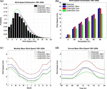
Figure 5 shows 10 m wind speed data at the nine synoptic stations for observed, CLM3-ERA 18 km, CLM3-ERA 7 km and CLM4-ERA 7 km resolution data for the period 1981–2000. Figure 5(a) compares the model wind speed distributions

Table III. The RMSE and MAD statistics for Test 1.

Station

CLM3 18 km CLM3 7 km CLM4 7 km

RMSE MAD RMSE MAD RMSE MAD

Belmullet 2.65 2.03 _{2.59 2.0 2.59 2.0}

Claremorris _{2.11 1.63} 2.41 1.89 2.23 1.75

Shannon 2.05 1.55 3.54 2.84 2.18 1.68

Valentia 3.25 2.61 2.75 2.17 2.34 1.80

Cork _{2.12 1.61} 2.23 1.70 2.44 1.84

Mullingar 2.24 1.79 2.81 2.31 _{2.22 1.78}

Dublin 2.16 1.64 2.23 1.70 2.29 1.75

Casement 2.68 2.08 2.47 1.89 2.66 2.04

Rosslare 3.26 2.58 2.60 2.0 _{2.46 1.89}

9 stations total 2.53 1.94 2.65 2.05 _{2.39 1.84}

The best scores are in bold face. The model data were bilinearly interpolated onto the latitude–longitude station location.

(a) (b)

(c) (d)

with the observed distribution. The CLM3-ERA 18 km and CLM3-ERA 7 km distributions show a positive bias in the probability of obtaining higher wind speeds, whereas the CLM4-ERA 7 km simulation shows a negative bias. This is reflected in Figure 5(b) the wind speed percentiles, (c) the mean monthly wind speed and (d) the diurnal cycle where, although we have good agreement, the CLM3-ERA 18 km and CLM3-ERA 7 km data overestimate whereas the CLM4-ERA 7 km data underestimate the wind speeds. To investigate if the results of Table III and Figure 5 are influenced by the difference in temporal resolution of the 18 and 7 km simulations (6 vs. 1 h), the evaluations were repeated for 7 km data at 6 h temporal resolution. It was found that the change in temporal resolution had only a marginal effect on the evaluation results.

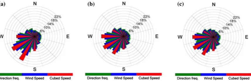
To investigate the ability of CLM to simulate the energy content of the wind, we consider the cube of the 10 m wind speed in Figures 6 and 7. The 10 m power wind roses at nine synoptic stations are shown in Figure 6 for (a) observed, (b) CLM3-ERA 7 km and (c) CLM4-ERA 7 km data. The power wind rose shows the directional frequency (green seg-ments), the contribution of each sector to the total mean wind speed (blue segments) and the contribution of each sector to the total mean cube of the wind speed (red segments). Figure 6 shows that the observed, CLM3-ERA 7 km and CLM4-ERA 7 km power wind roses are in close agreement, with the wind direction, speed, and power segments mostly having a south to west-north-west contribution.

Figure 7 shows a contour plot of the diurnal cycle of mean cube 10 m wind speed per month at the nine synoptic stations shown in Figure 1. The CLM3-ERA 18 km and CLM3-ERA 7 km data are in best agreement with observations. However, both simulations overestimate the mean cube wind speed, particularly during winter. The CLM4-ERA 7 km simulation shows a large negative bias because of its inability to estimate wind speeds at the higher scale.

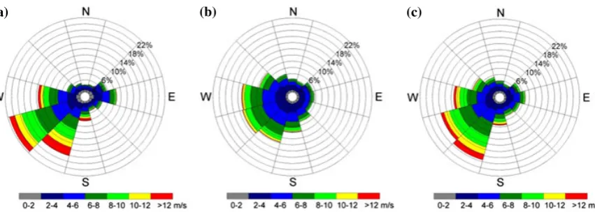
Table III and Figure 5 show that the CLM3-ERA 18 km simulation gives better results than the CLM3-ERA 7 km sim-ulation and is comparable with the CLM4-ERA 7 km simsim-ulation. However, when we look at individual locations, we see that the higher resolution simulations show better skill in simulating the detail and pattern of the wind climate, introduced by the local topography. This is evident in Figure 8: the 10 m wind roses at Casement Aerodrome which is located north of the Wicklow Mountains (Figure 1). The observed wind rose in Figure 8(a) demonstrates that the mountains act as a barrier, preventing south and south-easterly winds. This is better represented by the CLM3-ERA 7 km simulation. The CLM3-ERA 18 km simulation underestimates the south-westerly and easterly wind. The CLM4-ERA 7 km wind rose (not shown) is similar to the CLM3-ERA 7 km wind rose.

It is noted that the CLM evaluation simulations all show systematic patterns of error. It is difficult to determine which simulation performs best as results vary with the method of evaluation. For example, when comparing the wind speed with observations, the CLM4-ERA 7 km simulation gives the lowest MAD and RMSE values. However, it performs poorly at capturing high wind speeds and is therefore unable to accurately reproduce the mean cube wind speed. The CLM3-ERA 18 km validations sometimes show improvements over the 7 km simulations. However, as seen from the wind roses in Figure 8, the 7 km simulations perform better at simulating the detail and pattern of the wind climate, introduced by the local topography. This variation in model skill stresses the importance of using an ensemble of RCMs to simulate the climate.

4.2. Test 2: comparing the control and evaluation 7 km simulations

The CLM3-EC5_1 and CLM3-EC5_2 mean 10 m wind speed winds (not shown) were found to show qualitatively good agreement with the CLM3-ERA mean wind speed (Figure 3(b)) in terms of the spatial patterns and magnitude of the wind speed. Similarly, the CLM4-EC5_1 and CLM4_EC5_2 data were in good agreement with the CLM4-ERA data. The dif-ference plots in Figure 9 show a positive bias in the 10 m wind speed over Ireland of between 0 and 0.2 m s1for the

(a) (b) (c)

Figure 6.The 10 m power wind roses at nine synoptic stations (1981–2000): (a) observed, (b) CLM3-ERA 7 km and (c) CLM4-ERA 7 km. The power wind rose depicts the directional frequency, the contribution of each sector to the total mean wind speed and the

Figure 7.The annual diurnal 10 m mean cubed wind speed at nine stations is shown for (a) observation, (b) CLM3-ERA 18 km, (c) CLM3-ERA 7 km and (d) CLM4-ERA 7 km data.

(a) (b) (c)

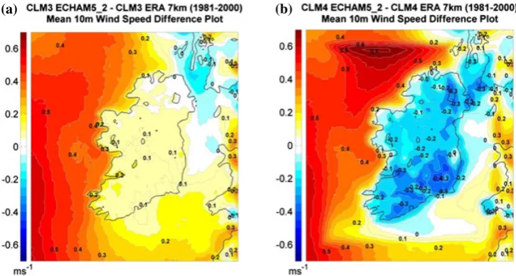
CLM3-EC5_2 simulation and a negative bias of between 0.1 and 0.2 m s1for the CLM4-EC5_2 simulation. Similarly, the difference plots (not shown) for the CLM3-EC5_1 and CLM4-EC5_1 simulations show a positive bias of between 0 and 0.3 m s1and a negative bias of between 0 and 0.3 m s1, respectively. The differences demonstrate the influence of the global climate driving data on the downscaled regional climate model and also provide an impression of the potential variability of the climate simulations. Since the differences observed in Figure 9 are comparable in magnitude with similar comparisons of the CLM3 18 km driving data,34this confirms the robustness of the CLM model in simulating the Irish climate. Table IV shows the MAD and RMSE statistics for test 2, calculated over the whole model domain. The boundary disturbances seen in Figure 9(b) (absent in Figure 9(a)) may be attributed to differences in the width of the lateral boundary relaxation zone of the CLM3 and CLM4 configurations of the present study.

4.3. Test 3: future climate predictions of the CLM model

The projected percentage change in the annual 60 m mean wind speed for all CLM 7 km SRES simulations was found to show no substantial increase or decrease over Ireland. In order to investigate the effects of climate change on the energy content of the wind, the projected changes in the 60 m mean cube wind speed were calculated. Again, small changes (0–2%) were observed in the energy content of the wind for all the SRES simulations.

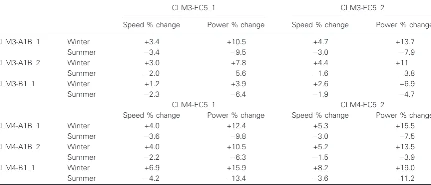
However, when stratified per season, we see substantial changes in the mean wind speed, particularly for the winter (December, January and February) and summer (June, July and August) months. Table V presents the projected changes over Ireland and a small area of the surrounding sea for all the CLM 7 km SRES comparisons. All projections show an expected increase in the 60 m winter mean wind speed over Ireland with values ranging from 1.2% to 8.2%. The projected change in the energy content of the 60 m wind for the winter months ranges from an increase of 3.9–19%.

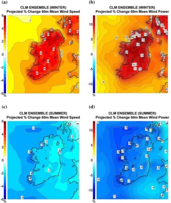
The projections all show an expected decrease in the 60 m summer mean wind speed over Ireland ranging from 1.5% to 4.2%. The projected change in the energy content of the wind for the summer months ranges from a decrease of 3.8–13.4%. Figure 10 shows the ensemble mean of the percentage changes in the 60 m mean wind speed and mean cube wind speed for winter and summer. Figure 10(a) shows an expected increase in the 60 m winter mean wind speed of between 3% and 5% over Ireland. The standard deviation of the ensemble of projected changes in mean winter wind speed (not shown)

(a) (b)

Figure 9. Mean 10 m wind speed difference (1961–2000): (a) CLM3-ECHAM5_2 minus CLM3-ERA and (b) CLM4-ECHAM5_2 minus CLM4-ERA.

Table IV. The MAD and RMSE statistics for Test 2.

MAD RMSE

CLM3-ERA vs. CLM3-EC5_1 0.34 0.39

CLM3-ERA vs. CLM3-EC5_2 0.24 0.30

CLM4-ERA vs. CLM4-EC5_1 0.33 0.39

ranges from 0.94% in the south of Ireland to 1% in the north. Figure 10(b) shows a projected increase of 6–13% in the energy content of the 60 m wind for the winter months over Ireland. The standard deviation of the ensemble of projected changes in energy content during winter (not shown) ranges from 3% in the north of Ireland to 8% in the south. Figure 10 (c) shows an expected decrease in the 60 m summer mean wind speed of between 2% and 3% over Ireland. The standard deviation of the ensemble of projected changes in mean summer wind speed (not shown) ranges from 0.84% in the north of Ireland to 0.94% in the south. Figure 10(d) shows an expected decrease of 5–8% in the energy content of the 60 m wind for the summer months over Ireland. The standard deviation of the ensemble of projected changes in energy content during summer (not shown) ranges from 2% to 4% over Ireland.

The statistical significance of changes in the 60 m wind speed is presented below. Since the projections in the annual mean wind speed over Ireland showed no substantial increase or decrease, the Ha0alternative hypothesis (described in

Section 3.6) is tested when analysing the statistical significance of changes in the annual wind speed. The test was applied to all the comparisons outlined in Table V. Results show that although some of the comparisons show significance at the 5% level over Ireland, most do not.

Since all projections show an increase over Ireland in the mean winter 60 m wind speed, the Ha2alternative hypothesis is

tested for the future winter projections. Here, the alternative hypothesis states that the future wind speeds are greater than the past. Results show that all comparisons showed high levels of significance over most of Ireland. Figure 11(a) shows the maximum confidence levelpof all 12 comparisons outlined in Table V. We see that the null hypothesis for all the CLM-EC5 SRES comparisons is consistently rejected over most of Ireland. We can conclude that the increase in future winter winds speeds over Ireland is statistically significant. The low levels of significance, observed in the north and north-west sector of the domain, correspond to small projected changes in the winter wind speed for three of the ensemble members. We see from Figure 11(b) that the decrease in the summer wind speed is significant over most of Ireland. Here, the alternative hypothesis states that the future wind speeds are less than the past.

In addition to projected changes in the mean wind speed, changes in the variability of the wind speed and the shape of the wind speed probability density function (pdf) are important for energy applications.

The standard deviation of the 60 m wind speed was calculated for each control and SRES future simulation. The percentage difference was then calculated for each comparison outlined in Table V. Figure 12 shows the mean of these percentage changes in the standard deviation of 60 m wind speed for winter and summer.

The fact that the future winter wind speed projections show an increase in both the mean and standard deviation suggests the future winter wind speed distributions are shifted to higher values (in the wind pdf) and have a larger spread. This is consistent with Figure 13(a); the past and future 60 m winter wind speed distributions at Arklow Wind Farm. This wind farm is Ireland’s largest offshore wind farm and is located approximately 10 km off the east coast (Figure 1). The future summer climate projections show a decrease in both the mean and standard deviation, suggesting the future summer wind speed distributions are shifted to lower values and have a smaller spread. This is consistent with Figure 13(b), the past and future 60 m summer wind speed distributions at Arklow Wind Farm.

To quantify the projected change in extreme wind speeds, the percentage change in the 60 m winter 99th percentiles was calculated for the comparisons outlined in Table V. All 12 comparisons showed a projected increase in the 99th percentile of 60 m winter wind speed over Ireland, of between 0% and 6%. The mean of these percentage changes is

Table V. The projected percentage change in the 60 m mean wind speed and mean cube wind speed for summer and winter.

CLM3-EC5_1 CLM3-EC5_2

Speed % change Power % change Speed % change Power % change

CLM3-A1B_1 Winter +3.4 +10.5 +4.7 +13.7

Summer 3.4 9.5 3.0 7.9

CLM3-A1B_2 Winter +3.0 +7.8 +4.4 +11

Summer 2.0 5.6 1.6 3.8

CLM3-B1_1 Winter +1.2 +3.9 +2.6 +6.9

Summer 2.3 6.4 1.9 4.7

CLM4-EC5_1 CLM4-EC5_2

Speed % change Power % change Speed % change Power % change

CLM4-A1B_1 Winter +4.0 +12.4 +5.3 +15.5

Summer 3.6 9.8 3.0 7.5

CLM4-A1B_2 Winter +4.0 +10.5 +5.2 +13.5

Summer 2.2 6.3 1.5 3.9

CLM4-B1_1 Winter +6.9 +15.9 +8.2 +19.0

Summer 4.2 13.4 3.6 11.2

presented in Figure 14, where an expected increase of 2–4.5% in extreme wind speed over Ireland is noted. The standard deviation of the ensemble of projected changes in the wind speed percentiles during winter ranges from 0.6% to 1.5% over Ireland (not shown).

Although substantial changes in the wind speed for the future winter and summer months are expected, it was noted that the general wind directions and wind speed spatial correlations did not show any considerable change.17

4.4. Test 4: comparison of the control simulations

Test 4 assesses the robustness of the climate change signal of test 3 by comparing the control simulations with each other. The climate change signal of test 3 shows an expected increase in mean wind speed for the future winter months and a decrease during summer. Accordingly, we compare the control simulations for winter and summer. Figure 15 compares the CLM4 EC5_1 with CLM4 EC5_2 simulation for winter (left) and summer (right). The percentage difference in the 60 m mean wind speed over Ireland ranges from 1% to 2% for winter and 0% to 1% for summer. The comparisons of CLM3 EC5_1 with CLM3 EC5_2 showed similar results. The magnitude of the percentage differences of test 4 are less than the climate change signal of Figure 10(a and c), thus increasing our confidence in the robustness of the climate change signal.

(c) (d)

(a) (b)

4.5. Test 5: comparison of the future projections

Test 5 assesses the robustness of the climate change signal of test 3 by comparing the CLM A1B_1 and CLM A1B_2 simulations with each other. Figure 16 compares the CLM3 A1B_1 with the CLM3 A1B_2 simulation for winter and summer. The percentage difference of the 60 m mean wind speed ranges from 0% to1% for winter and 0% to 2% for summer. The comparisons of CLM4 A1B_1 with CLM4 A1B_2 showed similar results. Figure 16(b) shows that over the south of Ireland, the test 5 results for summer are similar in magnitude to the climate change signal for summer (Figure 10(c)). The climate change signal for summer over the south of Ireland should therefore be viewed with caution. To address this issue, future work will focus on increasing the ensemble size. The magnitude of the percentage differences of test 5 are less than the climate change signal for winter (Figure 10(a)), thus increasing our confidence in the climate change signal for winter.

(a) (b)

Figure 11.Statistical signi_ficance of changes in the future 60 m wind speed using the Kolmogorov_–Smirnov test. The alternative hypothesis is accepted for small values ofp. (a) CLM ensemble winter and (b) CLM ensemble summer. Areas in thefigures that

are white indicate high levels of significance (p≪5%).

(a) (b)

5. CONCLUSIONS

We have examined the impact of simulated global climate change on the wind energy resource of Ireland using the method of regional climate modelling. In view of unavoidable errors due to model (regional and global) imperfections and the inherent limitation on predictability of the atmosphere arising from its chaotic nature, isolated predictions are of very limited value. To address this issue of model uncertainty, an ensemble of RCMs was run. The RCMs used were the CLM Community’s COSMO-CLM, versions 3.2 (CLM3) and 4.0 (CLM4). The Irish climate was simulated at 0.0625 (~7 km) spatial resolution.

(a) (b)

Figure 13.Comparing the CLM past and future 60 m wind speed distribution at Arklow Wind Farm shows (a) the winter distribution and (b) the summer distribution. The past distributions are calculated by combining the 60 m wind speeds of all the CLM EC5 7 km control simulations. Similarly, the future distributions are calculated by combining the 60 m wind speeds of all the CLM SRES 7 km simulations.

The research was undertaken to consolidate, and as a continuation of, similar research16using the Rossby Centre’s RCA3 RCM to investigate the effects of climate change on the future wind energy resource of Ireland. The RCA3 projections show a marked increase in the amplitude of the annual cycle in wind strength with 4–10% more energy available during winter and 5–14% less during summer. However, the uncertainty of the RCA3 projections was found to be high since the climate change signal was of similar magnitude to the variability of the evaluation and control simulations. The current research addresses this uncertainty by employing an ensemble of RCM simulations to study climate change. The issue of RCM uncertainty is assessed by employing different versions of COSMO-CLM to simulate the climate. To address the issue of inherent climate variability, the control and future simulations were repeated, using different realizations of the ECHAM5 data to drive the RCMs. Climate variability was then assessed by comparing the climate change signals with the variability of the control and future simulations. In addition, the COSMO-CLM model was run at a higher resolution than the RCA3 model, thus allowing us to better assess the local effects of climate change on the wind energy resource.

The CLM model was evaluated by performing past simulations of the Irish climate, driven at the lateral boundaries by ERA-40 data, and comparing the output to observations. The CLM3 7 km resolution simulation was found to overestimate

(a) (b)

Figure 15.The percentage difference of the 60 mean wind speed of the CLM4 EC5_2 and CLM4 EC5_1 simulations for (a) winter and (b) summer.

(a) (b)

the mean 10 m wind speed over Ireland by approximately 1–1.3 m s1. The CLM4 7 km simulation showed better results with a negative bias of approximately 0.1–0.2 m s1. It was noted that both CLM3 and CLM4 7 km data have a tendency not to capture wind speeds at the more extreme scales. This is particularly evident for the CLM4 data and results in a large negative bias in the CLM4 mean wind power data. These errors may be partially attributed to errors in the ERA-40 driving data. The consistent underestimation of wind speed by the CLM4 7 km simulations may be attributed to the use of the sub-grid scale orographic scheme36 as described in Section 3.1. The validation results are consistent with previous studies investigating the ability of the CLM model to accurately simulate windfields.34Separate studies, using different regional climate models, have also noted an inability of RCMs to accurately simulate high to extreme wind speeds for Ireland16and Northern Europe.7For example, most PRUDENCE42,43RCMs, although quite realistic over sea, severely underestimate the occurrence of very high wind speeds over land and coastal areas.44

For the investigation of the influence of the future climate under different climate scenarios, the Max Planck Institute’s GCM, ECHAM5, was used to drive the CLM models. Simulations were run for a control period 1961–2000 and future period 2021–2060. To add to the number of ensemble members, the control and future simulations were repeated using different realizations of the ECHAM5 data. The future climate was simulated using the two IPCC emission scenarios, A1B and B1. Future projections show a marked increase in the amplitude of the annual cycle in wind strength with 9–13% more energy available during winter and 5–8% less during summer.

To examine the robustness of the RCM projections, the climate change signals were compared with the variability of both the control and future simulations. Results show that over the south of Ireland, the variability in the future projections for summer is similar in magnitude to the climate change signal. The climate change signal for summer over the south of Ireland should therefore be viewed with caution. To address this issue, future work will focus on increasing the ensemble size. For winter, the variability of the control and future projections was found to be less than the climate change signal, thus increasing our confidence in the winter projections.

The projected changes for summer and winter were found to be statistically significant over most of Ireland. The future projections of wind direction and spatial correlations did not show any substantial change. An increase in extreme wind speeds is expected during winter, which may impact on the continuity of supply of wind power. Nevertheless, the simula-tion results show an expected increase in the frequency of wind speeds in the energetically useful range occurring during the winter months.17

The agreement of the COSMO-CLM results of the present study and the RCA3 results16increases our confidence in the robustness of the projections.

Regardless of this agreement, it is felt that the ensemble size of 12 of the current study is not large enough to accurately estimate the probability density function of predicted changes in future wind speed. Future research will focus on increasing the RCM ensemble size, thus increasing our confidence in the robustness of the projections. Additionally, the accuracy and usefulness of the model predictions can be enhanced by employing more up-to-date RCMs, GCMs and greenhouse gas scenarios. This work is already underway; the WRF45and COSMO-CLM RCMs are currently being used to downscale the HadGEM2-ES, CanESM2 and EC-EARTH CMIP546GCMs. The three representative concentration pathways, RCP4.5, RCP6 and RCP8.5 greenhouse gas concentration trajectories,47have been selected for the investigation of the future climate.

ACKNOWLEDGEMENTS

This research was supported and funded by the Environmental Protection Agency CCRP STRIVE Programme. We would like to thank the model and data group at Max Planck Institute for Meteorology in Hamburg, Germany for the ECHAM5-OM1 data and the CLM Community for the CLM model and for allowing access to the CLM3 18 km data. The ECMWF is acknowledged for allowing access to the ERA-40 data. The support received from Met Éireann, particularly from the Climate and Observations Division, is also gratefully acknowledged. We would also like to acknowledge the reviewers’assistance in greatly improving the paper.

REFERENCES

1. Troen I, Petersen EL. European Wind Atlas. Risø National Laboratory for the Commission of the European Communities: Roskilde, 1989; 656.

2. Frank HP, Landberg L. Modelling the wind climate of Ireland.Boundary-Layer Meteorology1997;85: 359–378. 3. SEI: Wind Atlas 2003 (Report No. 4Y103A-1-R1). Available: http://www.sei.ie/uploadedfiles/RenewableEnergy/

IrelandWindAtlas2003.pdf. (Accessed 31 August 2012)

5. Giorgi F. On the simulation of regional climate using a limited area model nested in a general circulation model.

Journal of Climate1990;3: 941–963.

6. Giorgi F. Regional climate modeling: status and perspectives.Journal de Physique IV2006;139: 101–118. DOI: 10.1051/jp4:2006139008.

7. Christensen JH, Hewitson B, Busuioc A, Chen A, Gao X, Held I, Jones R, Kolli RK, Kwon WT, Laprise R, Magaña Rueda V, Mearns L, Menéndez CG, Räisänen J, Rinke A, Sarr A, Whetton P. Regional climate projections. InClimate Change 2007: The Physical Science Basis. Contribution of Working Group I to the Fourth Assessment Report of the Intergovernmental Panel on Climate Change.Solomon S, Qin D, Manning M, Chen Z, Marquis M, Averyt KB, Tignor M, Miller HL(eds.). Cambridge University Press: Cambridge, United Kingdom and New York, NY, USA, 2007. 8. Warner TT, Peterson RA, Treadon RE. A tutorial on lateral boundary conditions as a basic and potentially serious

limitation to regional numerical weather prediction. Bulletin of the American Meteorological Society 1997; 78: 2599–2617.

9. Staniforth A. Regional modeling: a theoretical discussion.Meteorology and Atmospheric Physics1997;63: 15–29. 10. Miguez-Macho G, Stenchikov GL, Robock A. Regional climate simulations over North America: interaction of local

processes with improved large-scaleflow.Journal of Climate2005;18(8): 1227.

11. Giorgi FL, Mearns O. Introduction to special section: regional climate modeling revisited.Journal of Geophysical Research1999;104(D6): 6335–6352.

12. Qian JH, Seth A, Zebiak S. Reinitialized versus continuous simulations for regional climate downscaling.Monthly Weather Review2003;131: 2857–2874.

13. Lo JCF, Yang ZL, Pielke Sr. RA. Assessment of three dynamical climate downscaling methods using the weather research and forecasting (WRF) model. Journal of Geophysical Research 2008; 113: D09112. DOI: 10.1029/ 2007JD009216.

14. Chen F, Janjic ZI, Mitchell K. Impact of atmospheric surface-layer parameterizations in the new land-surface scheme of the NCEP mesoscale eta model.Boundary Layer Meteorology1997;85: 391–421.

15. Rockel B, Will A, Hense A. The regional climate model COSMO-CLM (CCLM).Meteorologische Zeitschrift2008; 17(4): 347–348.

16. Nolan P, Lynch P, McGrath R, Semmler T, Wang S. Simulating climate change and its effects on the wind energy resource of Ireland.Wind Energy2011, DOI: 10.1002/we.489.

17. Nolan P. Simulating climate change and its effects on the wind energy resource of ireland. 2009, PhD Thesis: http:// mathsci.ucd.ie/met/staff/PaulNolan/PhD_Thesis_Paul_Nolan.pdf. (Accessed 31 August 2012)

18. Jones CG, Willén U, Ullerstig A, Hansson U. The Rossby Centre regional atmospheric climate model part I: model climatology and performance for the present climate over Europe.Ambio2004;33: 199–210.

19. Samuelsson P, Gollvik S, Ullerstig A. The land-surface scheme of the Rossby Centre regional atmospheric climate model (RCA3). Report in Meteorology122, SMHI. SE-601 76 Norrköping, Sweden, 2006; 43.

20. Roeckner E, Bauml G, Bonaventura L, Brokopf R, Esch M, Giorgetta M, Hagemannn S, Kirchner I, Kornblueh L, Manzini E, Rhodin A, Schlese U, Schulzweida U, Tompkins A. The atmospheric general circulation model ECHAM5 part I: model description, Max-Planck Institute for Meteorology, report no. 349, Hamburg, Germany. 2003; 1–127. 21. IPCC.Special Report on Emission Scenarios. A Special Report of Working Group III of the Intergovernmental Panel

on Climate Change. Nakicenovic N, Swart S (eds.). Cambridge University Press: Cambridge, UK, 2000; 599. 22. IPCC. In Climate Change 2007: The Physical Science Basis. Contribution of Working Group I to the Fourth

Assessment Report of the Intergovernmental Panel on Climate Change. Solomon S, Qin D, Manning M, Chen Z, Marquis M, Averyt KB, Tignor M, Miller H (eds.). Cambridge University Press: Cambridge and New York, NY, 2007. 23. Semmler T, Varghese S, McGrath R, Nolan P, Wang S, Lynch P, O’Dowd C. Regional model simulation of North Atlantic cyclones: present climate and idealized response to increased sea surface temperature.Journal of Geophysical Research2008;113: D02107.

24. Geng Q, Sugi M. Possible change of extratropical cyclone activity due to enhanced greenhouse gases and sulphate aerosols—study with a high-resolution AGCM.Journal of Climate2003;16: 2262–2274.

25. Hall NMJ, Hoskins BJ, Valdes PJ, Senior CA. Storm tracks in a high resolution GCM with doubled carbon dioxide.

Quarterly Journal of the Royal Meteorological Society1994;120: 1209–1230. DOI: 10.1256/smsqj.51904.

26. Harrison GP, Cradden LC, Chick JP. Preliminary assessment of climate change impacts on the UK onshore wind energy resource.Energy SourcesSept 2008;30(14): 1286–1299.

28. Pryor SC, Barthelmie RJ. Climate change impacts on wind energy: a review. Renewable and Sustainable Energy Reviews2010;14: 430–437.

29. Breslow PB, Sailor DJ. Vulnerability of wind power resources to climate change in the continental United States.

Renewable Energy2002;27: 585–98.

30. Sailor DJ, Smith M, Hart M. Climate change implications for wind power resources in the Northwest United States.

Renewable Energy2008;33: 2393–2406.

31. Doms G, Schättler U. A description of the nonhydrostatic regional model LM. Part I: dynamics and numerics, Deutscher Wetterdienst, Offenbach. 2002; 134. Available: www.cosmo-model.org. (Accessed 31 August 2012) 32. Steppeler J, Doms G, Schättler U, Bitzer HW, Gassmann A, Damrath U, Gregoric G. Meso-gamma scale forecasts

using the nonhydrostatic model LM.Meteorology and Atmospheric Physics2003;82: 75–96.

33. Keuler K, Radtke K, Georgievski G. Summary of evaluation results for COSMO-CLM version 4.8_clm13 (clm17): comparison of three different configurations over Europe driven by ECMWF reanalysis data ERA40 for the period 1979–2000. 2012; Available: http://www.clm-community.eu/dokumente/upload/34daa_Evaluation-report_CCLM_4.8_v8.pdf. (Accessed 31 August 2012)

34. Hollweg HD, Böhm U, Fast I, Hennemuth B, Keuler K, Keup-Thiel E, Lautenschlager M, Legutke S, Radtke K, Rockel B, Schubert M, Will A, Woldt M, Wunram C. Ensemble simulations over Europe with the regional climate model CLM forced with IPCC AR4 global scenarios Hamburg: Max-Planck-Institut für Meteorologie, Gruppe Modelle und Daten 2008. 150. CLM Technical Report 3. Available: www.mad.zmaw.de/fileadmin/extern/documents/reports/ MaD_TechRep3_CLM__1_.pdf. (Accessed 31 August 2012)

35. Davies HC, Turner RE. Updating prediction models by dynamical relaxation: an examination of the technique.

Quarterly Journal of the Royal Meteorological Society1977;103: 225–245.

36. Lott F, Miller MJ. A new subgrid-scale orographic drag parametrization: its formulation and testing.Quarterly Journal of the Royal Meteorological Society1997;123: 101–127.

37. Uppala SM, Allberg K, Simmons PW, Andrae AJ, Da Costa U, Bechtold V, Fiorino M, Gibson JK, Haseler J, Hernandez A, Kelly GA, Li X, Onogi K, Saarinen S, Sokka N, Allan RP, Andersson E, Arpe K, Balmaseda MA, Beljaars ACM, Van De Berg L, Bidlot J, Bormann N, Caires S, Chevallier F, Dethof A, Dragosavac M, Fisher M, Fuentes M, Hagemann S, Holm E, Hoskins BJ, Isaksen L, Janssen PAEM, Jenne R, Mcnally AP, Mahfouf JF, Morcrette JJ, Rayner NA, Saunders RW, Simon P, Sterl A, Trenberth KE, Untch A, Vasiljevic D, Viterbo P, Woollen J. The ERA-40 re-analysis.Quarterly Journal of the Royal Meteorological Society2005;131: 2961–3012.

38. Model information of potential use to the IPCC lead authors and the AR4, January 2005. Available: http://www-pcmdi. llnl.gov/ipcc/model_documentation/ECHAM5_MPI-OM.pdf. (Accessed 31 August 2012)

39. Doms G, Schättler U. A description of the nonhydrostatic regional model LM. Part I: user’s guide, Offenbach. 2002; 134. Available: www.cosmo-model.org. (Accessed 31 August 2012)

40. Hollander M, Wolfe DA.Nonparametric Statistical Methods. Wiley: Hoboken, NJ, 1973.

41. Gibbons JD.Nonparametric Statistical Inference(2nd edn). Marcel Dekker: New York, NY, 1985.

42. Christensen JH, Carter TR, Rummukainen M, Amanatidis G. Evaluating the performance and utility of regional climate models: the PRUDENCE project.Climatic Change2007; DOI:10.1007/s10584-006-9211-6.

43. Déqué M, Jones RG, Wild M, Giorgi F, Christensen JH, Hassell DC, Vidale PL, Rockel B, Jacob D, Kjellström E, de Castro M, Kucharski F, van den Hurk B. Global high resolution versus Limited Area Model climate change scenarios over Europe: results from the PRUDENCE project.Climate Dynamics2005;25(6): 653–670. DOI: 10.1007/s00382-005-0052-1, ISSN 0930-7575.

44. Rockel B, Woth K. Future changes in near surface wind speed extremes over Europe from an ensemble of RCM simulations.Climatic Change2007; DOI: 10.1007/s10584-006-9227-y.

45. Skamarock WC, A description of the advanced research WRF version 3. NCAR Tech. Note NCAR/TN-475+STR. 2008; 113. Available: http://www.mmm.ucar.edu/wrf/users/docs/arw_v3.pdf. (Accessed 31 August 2012)

46. WCRP coupled model intercomparison project—phase 5: special issue of the CLIVAR Exchanges Newsletter, 2011, No. 56, Vol. 15, No. 2.