On the Sources of Heterogeneity in Banking Efficiency Literature

(1)

Munich Personal RePEc Archive

On the Sources of Heterogeneity in

Banking Efficiency Literature

Aiello, Francesco and Bonanno, Graziella

Department of Economica, Statistics and Finance, Unical, Italy,

Royal Docks Business School, University of East London, London

12 September 2014

Online at

https://mpra.ub.uni-muenchen.de/68300/

(2)

1

On the Sources of Heterogeneity in

Banking Efficiency Literature



Francesco Aiello

a

_{, Graziella Bonanno}

a,b

[email protected] - [email protected]

a_{Department of Economics, Statistics and Finance, University of Calabria}

I-87036, Arcavacata di Rende (CS), Italy

b_{Royal Docks Business School, University of East London, Docklands Campus} 4-6 University Way, London E16 2RD, UK

Abstract One learns two main lessons from studying the great quantity of banking efficiency literature. These lessons regard the heterogeneity in results and the absence of a comprehensive review aimed at understanding the reasons for this variability. Surprisingly, although this issue is well-known, it has not been systematically analyzed before. In order to fill this gap, we perform a Meta-Regression-Analysis (MRA) by examining 1,661 efficiency scores retrieved from 120 papers published over the period 2000-2014. The meta-regression is estimated by using the Random Effects Multilevel Model (REML), because it controls for within-study and between-study heterogeneity. The analysis yields four main results. Firstly, parametric methods yield lower levels of banking efficiency than nonparametric studies. This holds true even after controlling for the approach used in selecting the inputs and outputs of the frontier. Secondly, we show that banking efficiency is highest when using the value added approach, followed by estimates from studies based on the intermediation method, whereas those based on the hybrid approach are the lowest. Thirdly, efficiency scores also depend on the quality of studies and on the number of observations and variables used in the primary papers. As far as the effects of sample size, dimension and quality of papers are concerned, there are significant differences in sign and magnitude between parametric and nonparametric studies. Finally, cost efficiency is found to be higher than profit and production efficiency. Interestingly, MRA results are robust to the potential outliers in efficiency and sample size distributions.

JEL classification: C13, C14, C80, D24, G21, L25

Keywords: Banking industry, Frontier Models, Efficiency, Meta-analysis, Study design

1. Introduction

The understanding of how, or indeed whether, banks are efficient is one of the most intriguing fields of research in economics. The reason for this lies mainly in the fact that banking fosters economic growth (Bumann et al., 2013; Pagano, 1993; Raghuram et al., 1998) and, thus, studying efficiency becomes a crucial issue in the discipline. Furthermore, the demand for

_{The authors would like to thank Kristiaan Kerstens, Sergio Destefanis, Giovanni D}_’_{Orio, Damiano}

(3)

2

efficiency studies has increased over time because the results inform policy decisions and influence individual behavior. Within the context of our subject, this implies that stakeholders (policy-makers, regulators, investors and private agents) wish to know how banks could perform better, remain on the frontier and ensure financial market stability. To some extent, these reasons explain why, since the 1990s, many countries have regulated their national banking systems with the aim of increasing _banks’efficiency. From this point of view, banking has become an interesting case-study for evaluating the effectiveness of any restructuring process, such as deregulation or M&A. On this basis, efficiency is the main concern in many policy-oriented papers.

Moreover, the growing attractiveness of efficiency studies is also driven by various methodological concerns. The theory of production clearly explains whether a decision unitis efficient or not. Farrell (1957) conceptualized technical (TE) and allocative efficiencies (AE) as part of overall efficiency (EE), with EE=TE*AE. In our case, TE represents banks_’ ability to produce maximum ou_{tput given a set of inputs and technology, while AE measures banks’} success in choosing their optimal input combinations. However, controversy has surrounded the empirics of many efficiency papers, with the result that the question, _{“What is the best} banking frontier and how can it be properly estimated?”, still awaits a conclusive answer. This is due to the fact that the frontier is unknown and that estimating approaches differ from one another in several ways, with no consensus on the superiority of one method over the others (Berger and Humprey, 1997; Coelli and Perelman, 1999; Fethi and Pasourias, 2010).

This said, the main consequences of the increased interest in banking efficiency are (a) an impressive proliferation of empirical research and (b) a relevant heterogeneity in results, even for narrowly defined topics. The highly mixed evidence is due to the variety of study designs underlying each work: researchers have to choose between parametric and nonparametric methods, stochastic and deterministic approaches, functional forms to be assigned to the frontier, and distributions for errors and efficiency. Variability is further caused by the econometrics used in estimating the frontiers and also depends on sample size and the number of inputs and outputs. Another factor explaining differences relates to the spam-period covered in the study. While the above remarks are valid for all works on efficiency, whatever the industry, a sector specific source of heterogeneity exists in banking literature. This regards how deposits are treated: the extreme options are the value added and the intermediation approaches which basically differ in that the former considers deposits as output, while the latter considers them as input. In short, it is not surprising that all this heterogeneity in the empirical setting of each paper translates into heterogeneity in efficiency scores.

(4)

3

find that the two methods provide efficiency scores which have statistically different means. Other valuable descriptions of how efficiency scores are sensitive to estimation methods are provided by Casu and Girardone (2004), Huang and Wang (2002), Kumar and Arora (2010), Mobarek and Kalonov (2014) and Yildirim and Philippatos (2007).

Besides the single studies which have tried to compare the results that different methods yield from a fixed sample of banks, some authors have reviewed the literature (Berger, 2007; Berger and Humphrey, 1997; Fethi and Pasiouras, 2010; Paradi and Zhu, 2013). While these surveys offer detailed and extremely valuable arguments about the reliability of results and why they may differ, none of them quantifies the impact of methodological choices on the variability of efficiency scores. A response to this issue may be provided by Meta-Analysis (henceforth MA), which is a statistical method used to collect and integrate the results from individual papers with the aim of evaluating whether, and to what extent, the features of each work (i.e. estimation method, year of publication, functional form assigned to frontier, sample size, and dimension) affect the findings (Stanley, 2001). As Glass

(1976) says, MA “connotes a rigorous alternative to the casual, narrative discussions of research studies which typify our attempt to make sense of the rapidly expanding research

literature” (Glass, 1976, 3).

Even though MA was originally applied to other disciplines, such as medicine and psychology (Egger et al., 1997; Hedges and Olkin, 1985; Rosenthal, 1984), it has recently been used in a number of papers covering a very wide spectrum of economic subjects (cfr. footnote 2). As far as efficiency literature is concerned, the prevalent interest is in summarizing the case of efficiency in agriculture, as in Bravo-Ureta et al. (2007), Thiam et al. (2001) and Kolawole (2009). Other excellent applications of MA to efficiency include those carried out by Brons et al. (2005), focusing on urban transport, and Odeck and Bråthen (2012), who summarize the technical efficiency literature regarding seaports. Nguyen and Coelli (2009) analyze the health sector.

Given the increased interest in MA and the fact that the literature on banking industry efficiency lends itself well to being summarized through this approach (the richness of sources behind the great heterogeneity in results is extremely high), it is noteworthy that no exhaustive work has explored the “banking efficiency-study design” nexus. In attempting to fill this gap, this paper considers large sample of efficiency studies and tests the robustness of results to different specifications of MA regressions.

A broadly similar study to ours is that by _{Iršová and Havránek (2010)}, which, however, focuses exclusively on the US banking system. Their MA refers to the period 1977-1997 and considers 32 papers, yielding a maximum of just 59 observations for some regressions and even fewer for others. Despite the limited sample size, they argue that the methodology adopted affects the efficiency scores. However, they realize that their “findings still need to be

verified by future research using a broader sample of empirical studies” (Iršová and

Havránek, 2010, 319).

Bearing in mind that some key elements (the number of stu

dies

covered,

(5)

4

size and the sign of the impact on the estimated efficiency scores brought about by different methodological choices made by authors of primary papers. The general question we ask is how much the efficiency scores are systematically influenced by the study design in the original papers. To be more precise, the scope of the research is to address these main issues. Whether parametric studies yield different results from nonparametric studies. Whether

different approaches regarding the variables to be included into banks’ frontiers have an impact on the average level of efficiency. Whether the impacts differ when considering cost instead of profit or production efficiency. Whether results change over time. What the consequences are of country-specific factors on national banking systems.

The rest of the paper is organized into 7 sections. Section 2 summarizes the methods most commonly used to estimate efficiency. Section 3 briefly presents MA, while section 4 reviews MA applications to economics and efficiency. Section 5describes the criteria adopted to create the meta-dataset and highlights the efficiency heterogeneity of primary studies. Section 6 presents and discusses the results. Section 7 concludes.

2. Measuring efficiency: main features

While the concept of efficiency is subject to different interpretations (Aigner et al., 1977; Battese et al., 2005; Farrell, 1957), there is consensus in considering efficiency to be the degree of proximity of an actual production process to a standard of optimality. Efficiency can be thought of as the ability of a decision unit to minimize the amount of input for the production of a certain output (input-oriented TE) or to maximize the amount of output given a certain amount of input (output-orientated TE), for any level of technology. Furthermore, efficiency may be evaluated and interpreted from different perspectives, depending on whether the focus is on production, profits, costs or revenues.

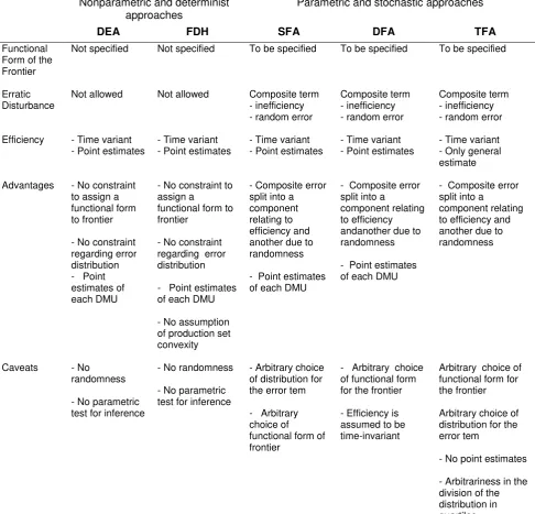
Since efficiency is evaluated in relation to the best-practice, the key concerns in this field of research come from the methods applied to estimate the frontier. Table 1 summarizes these methods. The proposed classification reports, method by method, the requirements regarding the functional form to be assigned to the frontier, the assumptions regarding the disturbances (existence and composition) and some specificities of the efficiency scores (time-invariant, punctual estimates). A number of advantages/caveats are highlighted for each technique.

(6)

5

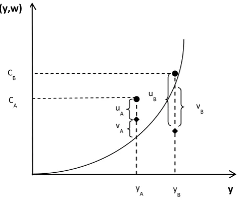
refer to banking industry by considering a cost function C(y,w) to produce output y at some price of input w. There are two banks, A and B, for which we observe the costs CA and CB of producing YA and YB respectively. When analyzing bank A by using a deterministic method, DEA for instance, the level of inefficiency is given by uA + vA, the entire distance from the frontier, while SFA admits randomness, e.g. vA, and, therefore, yields an inefficiency score of just uA. In this case, DEA over-evaluates inefficiency. In the case of bank B, an unforeseen positive disturbance, vB, makes the inefficiency obtained by applying SFA equal to uB, i.e. higher than that obtained through DEA. From this discussion, the crucial point to be emphasized is that the sign of random errors may be negative, a situation that is not taken into account when using DEA. Figure 1 makes it clear that it is not certain that DEA will underestimate efficiency with respect to SFA, as is intuitively to be expected, since DEA treats the distance from the frontier as inefficiency, while SFA allows for noise. The final net result depends on the type of adjustment made for the erratic component (see also Nguyen and Coelli, 2009).

Table 1 highlights the fact that there are numerous different ways to perform an efficiency study and that, despite the high degree of specialization in the use of various methods, the effect of some methodological choices is still not certain. For example, we learn from figure 1 that the estimated efficiency scores in stochastic methods may be higher or lower than those obtained using the deterministic approach. Similarly, much may be said with regards other options to be made. The following brief considerations come from in-depth discussions concerning the advantages and limitations of the methodological choices to be made when measuring efficiency (Berger and Humphrey, 1997; Coelli, 1995; Fethi and Pasourias, 2010; Nguyen and Coelli, 2009). For instance, the orientation of deterministic models (input versus output-oriented) and the distribution of efficiency in stochastic parametric models are two additional factors with an uncertain impact on efficiency. On the other hand, the use of panel data would generate higher efficiency levels than those from cross-section. An analogous impact is expected when using second order functional forms instead of the Cobb-Douglas. Finally, efficiency would increase with the number of variables included in the frontier, while it would decrease with small sample-size and the assumption of constant returns to scale. However, while the theory predicts the likely impact of any choice, the actual measure of how the results are sensitive to the study design is an issue to be addressed empirically. To thisend, this paper focuses on banking efficiency literature.

(7)

[image:7.595.55.542.125.592.2]

6

Table 1 A breakdown of some methods used to estimate efficiency

Legend: DEA = Data Envelopment Analysis; FDH = Free Disposal Hall; SFA: Stochastic Frontier

Approach; DFA = Distribution Free Approach; TFA = Thick Frontier Approach. Nonparametric and determinist

approaches

Parametric and stochastic approaches

DEA FDH SFA DFA TFA

Functional Form of the Frontier

Not specified Not specified To be specified To be specified To be specified

Erratic Disturbance

Not allowed Not allowed Composite term - inefficiency - random error

Composite term - inefficiency - random error

Efficiency - Time variant - Point estimates

- Time variant - Point estimates

- Time variant - Only general estimate

Advantages - No constraint to assign a functional form to frontier

- No constraint regarding error distribution - Point estimates of each DMU

- No constraint to assign a

functional form to frontier

- No constraint regarding error distribution

- Point estimates of each DMU

- No assumption of production set convexity

- Composite error split into a component relating to efficiency and another due to randomness

- Composite error split into a

component relating to efficiency andanother due to randomness

- Composite error split into a

component relating to efficiency and another due to randomness

Caveats - No randomness

- No parametric test for inference

- No randomness

- No parametric test for inference

- Arbitrary choice of distribution for the error tem

- Arbitrary choice of functional form of frontier

- Arbitrary choice of functional form for the frontier

- Efficiency is assumed to be time-invariant

Arbitrary choice of functional form for the frontier

Arbitrary choice of distribution for the error tem

- No point estimates

(8)

7

u

B

v

B

C(y,w)

y

u

A

v

A

y

B

y

A

C

B

C

[image:8.595.175.413.110.310.2]

A

Figure 1 The distance from the frontier: comparing SFA and DEA

3. The Meta-Analysis in a nutshell

The difficulty of comparing the results of empirical works is a common caveat in economics because studies differ in several ways. As discussed above, the main source of heterogeneity is the study design, but differences also depend on time periods covered, samples and data source used in each analysis. Another source of heterogeneity in final outcomes lies in the changes to contextual and institutional factors that potentially affect any decision unit.

One approach which deals with this heterogeneity in results is the Meta Regression Analysis (Glass, 1976; Glass et al., 1981; Stanley and Jarrell, 1989). MA is a statistical method which reveals more about a significant phenomenon that has been studied in a large set of empirical works. It investigates the relationship between the dependent variable (i.e. the principle finding of the primary studies covered in the MA) and some features of every paper. By modeling all of the relevant differences across studies of a given subject, MA allows us to assess the role of each varying factor in determining the variability in outcomes. In other words, MA provides a systematic synthesis of a substantial number of studies and stresses the quantitative effect of various relevant characteristics in the original papers in explaining the variability of results. In detecting the main sources of variability, MA offers the opportunity to direct future research.

In its essence, MA offers some advantages with respect to the standard qualitative literature surveys. Indeed, it does not suffer from potential bias in selecting the studies to be reviewed because it covers all of the relevant literature without restrictions accruing from the

reviewer’s judgments. As an extreme solution, when complete (or relatively wide) coverage is not feasible, MA mitigates any bias relating to the researcher’s preference by performing inferential analysis on a relatively representative randomized sample of the papers of interest. Our MA utilizes an exhaustive sample of papers and, therefore, ensures an ample coverage of the literature on banking efficiency (details on the original papers selected are in section 5).

(9)

8

different from one another. This is a sort of “apples and oranges problem” that can be addressed by refining the identification of the problem to be studied in order to focus attention on the specific factors that are assumed to be important in explaining differences in results. In this respect, this study only focuses on the few elements that are considered to be significant sources of variability in the estimations of banks_’ efficiency. For instance, the main point of interest is to understand how the use of nonparametric or parametric methods affects efficiency scores. One issue to be addressed regards whether banks perform better when maximizing profits than when controlling costs and whether results are statistically different when using the intermediation approach instead of the value added approach or a combination of both (the so-called hybrid approach).

Another potential limit is that MA assigns the same weight to the results of different works regardless of the quality of the studies. In this respect, it is also necessary to point out that one must also include working papers in order to obtain an appropriate coverage of studies and enrich the heterogeneity in results. Including all the literature makes sense because important information regarding the topic in question may be retrieved from unpublished, as well as published, papers. With the aim to address this issue, a binary variable for study quality is included, as in Disdier and Head (2008).1 _{We will control for quality of} publication by (i) using a dummy variable to distinguish between journal papers and works published as working papers and by (ii) using a continuous variable which we create by referring to the Impact Factor (IF) of each journal at the time of the publication of a primary paper.

Finally, MA may suffer from publication bias, in the sense that final results may reflect the fact that journals tend to publish papers whose evidence is robust in statistical terms. In order to control for this issue, many scholars weight the observations by using appropriate measures of the estimates_’ variability (Bumann et al., 2013; Cipollina and Salvatici, 2007; Doucouliagos and Stanley, 2009; Feld et al., 2013; Stanley, 2008). From an empirical perspective, these studies indicate that the Random Effect Multilevel Model (REML) and the weighted-cluster data analysis (WLS) are robust to publication bias. After controlling for publication bias in our sample, we will proceed by using the REML technique because it controls not only for within-study variability, but also for between-study heterogeneity (cfr. 6.1).

4. Meta-Analysis in efficiency literature

The use of MA is increasing in economics and is applied to a very wide range of areas. Poot (2012) counts 626 papers which applied MA to economics between 1980 and 2010, with an exponential growth in the 2000s. About three quarters of these MA applications were published in field-specific journals, several appeared in _“top_” journals (The American Economic Review, Journal of Banking and Finance, Journal of Political Economy, Review of Economics and Statistics, and The Economic Journal), whilst the remaining were disseminated across working papers or book chapters. Among other things, Poot (2012) shows that scholars have only paid attention to publication bias in the most recent MA studies.

Although there has been a widespread use of MA in many areas of economics,2_{it is} worth noting that few papers deal with efficiency and, when they do, most consider the

1_{Disdier and Head (2008) introduce a dummy variable equal to 1 if the study is published in one of the following} top three journals: the American Economic Review, the Journal of International Economics and Review of Economics and Statistics.

(10)

9

agricultural sector. For instance, Bravo-Ureta et al. (2007) examine the efficiency data collected from 167 farm level studies (569 observations) published over the last four decades. Their main results indicate that nonparametric deterministic models yield higher estimates of efficiency levels than stochastic frontier models do, whereas parametric deterministic frontiers yield lower estimates. Furthermore, the role of functional form is vague, while a significant effect is found for the structure of data used in the original papers, in the sense that cross-sectional data produce lower estimates than panel data. This is also found in Thiam et al. (2001), who review 34 articles covering agricultural efficiency in developing countries. The authors find that no effect on efficiency is exerted by the number of variables in the model, crop type, stochastic versus deterministic frontiers and sample size, while efficiency in agriculture increases with the number of fixed inputs and the number of inputs. Kolawole (2009) focuses on Nigerian agriculture3_{and performs an MA covering 64 studies and 86}

observations for the period 1999-2008. He shows that the sample size, the number of inputs used and the aggregate output variable (i.e., single output variable) are the main sources of variability in efficiency in Nigerian agriculture. The author also finds that crop and livestock production perform better than other agricultural sectors and that studies on the northeast and southeast regions of the country yield lower scores of efficiency. It is important to point out that the MA performed by Kolawole (2009) lacks, as the author acknowledges, _“published information on the study specific characteristics used as explanatory variables in the

regression” (p. 14).

While Brons et al. (2005) focus on urban transport, finding that there is no statistical difference in efficiency scores between parametric and nonparametric studies, Odeck and Bråthen (2012) analyze the variations in the technical efficiency of seaports using 40 published papers (127 estimates) and show significant differences between results obtained by using a variety of methods. One of the main findings is that the random effects model outperforms the fixed effects model in explaining variations in efficiency. Moreover, the estimated efficiency of recent studies is low compared with earlier published papers. Interestingly, DEA yields, on average, higher estimations of efficiency than SFA. Finally, efficiency increases when moving from studies based on panel data to cross-sectional analyses. Another MA is that carried out by Nguyen and Coelli (2009), who focus on hospital efficiency. They use 253 observations obtained from 95 primary studies published between 1987 and 2008. Their paper explains the differences in efficiency with respect to sample size, number of variables, parametric versus nonparametric method, returns to scale, functional

and consumer economics. In order to give an idea of the wide spectrum of recent MA applications in economics, it is sufficient to say that they have been used with regard such topics as the tax impact on corporate debt financing (Feld et al., 2013), the financial liberalization-growth nexus (Bumann et al., 2013), misalignments in real exchange rates (Ègert and Halpern, 2006), the demand for gasoline (Havranek et al., 2012), labor supply elasticities (Chetty et al., 2011), the relationship between FDI and taxation (Feld and Heckemeyer, 2011), the effect of active labor market policies (Card et al. 2010), aid effectiveness (Doucoliagos and Paldam, 2009), the role of distance in bilateral trade (Disdier and Head, 2008), the 2% _β-Convergence (Abreu et al., 2005) and a variety of other environmental and transport issues (summarized in van den Bergh and Button, 1997).

3_{According to the author, the decision to consider a single country helps to overcome the weakness} relating to the fact that, in Thiam et al. (2001) and Bravo-_{Ureta et al. (2007), “each cited study is} treated as an experiment based on a sample from a single population by implicitly assuming a common benchmark for the comparison: i.e., the existence of a population Is _{implicit in these studies. ………. the} advantage (to focus on a single country) is, in our view, more than outweighed by the easier

(11)

10

form, error distribution form, cost versus technical efficiency and cross-sectional versus panel data. The authors find that, in hospital efficiency literature, sample size and constant returns to scale have a negative effect on efficiency, while the number of variables exerts a positive effect. None of the other individual study features have an impact on efficiency.

A very similar research question to ours has been addressed by _{Iršová and Havránek} (2010) who review US banking efficiency literature covering the years from 1977 to 1997. Their dataset comprises 32 papers and 53 observations. By applying several estimators (OLS, Tobit, Iteratively re-weighted least squares method, and Random-Effect), they show that US banks are less efficient when generating profits than when controlling costs. Interestingly, when referring to the translog functional form, the estimated efficiency scores are high compared with the Fourier specification. In the words of Iršová and Havránek (2010):

“ … the functional forms generally operate in opposite directions (translog functional form positively and Fourier functional form negatively), which contradicts the results in Berger & Mester (1997) who favour an insignificant difference between these two forms. According to our results, the translog parametric choice does not _{return significantly different}results from the nonparametric approaches. Therefore, when _{researchers happen to find different} results between parametric and nonparametric approaches, it is mainly due to the usage of a Fourier-_{flexible production function” (p. 319).}

The paper by Iršová and Havránek (2010) is the only MA which has been conducted to review the efficiency studies in banking. However, it covers just one country, uses a sample of just a few papers and observations and the surveyed literature only considers papers focusing on US bank efficiency up to 1997, when in studying this literature we have observed, over the 2000s, a proliferation of scientific contributions employing a very wide spectrum of methods and focusing on very different samples of banking industry. Again, scholars refer to very different frameworks of analysis and use various econometric methods in order to address the research question. The choice of the estimation method is a key aspect in this class of study. In fact, the signs of the results and the existence of actual efficiency gains are not uniform. However, different works come to different conclusions, even when using the same type of estimation approach and, sometimes, when considering the same time period. Having said this, the lack of a systematic and quantitative survey on banking efficiency is surprising because MA fits the banking sector very well . The hypothesis that the heterogeneity in results may depend on the methodological choices of each study remains an interesting issue to be addressed empirically.

5. The Bank-Efficiency Meta Dataset

A delicate phase of an MA is the creation of the database. The number of potential papers in banking literature is impressive: for instance, when searching through _{Google for “banking}

efficiency”, one obtains more than 45,000 results (as of 24th_{April, 2014). This diminished to} 10,800 after controlling for “frontier”. Therefore, in order to collect a representative sample of works, we employ some criteria to identify relevant academic studies from the large pool of papers on bank efficiency.The search was conducted in two phases.

Firstly, we refer to the EconBiz, Repec, ScienceDirect, IngentaConnect and Econlit archives. The key-words used in the baseline search in the title, abstract or keywords are

(12)

11

performing of an MA (efficiency scores and standard deviations); (c) ran specific models for estimating the frontier (DEA, SFA, others); (d) were written in English; (f) were published in a journal or as working papers after 2000; (g) conducted analysis at bank (not branch) level. In this phase, we excluded the papers with the same efficiency score result as were reported in other papers by the same author/s and papers that do not report efficiency estimates.

Secondly, we (a) manually consulted the principal field journals (the Journal of Banking and Finance, Journal of Productivity Analysis, Review of Financial Studies, Journal of Financial Economics, European Journal of Operational Research, Applied Financial Economics and Journal of Business Finance & Accounting); (b) explored additional databases such as the Google Scholar and Social Science Research Network (SSRN) and (c) verified that we had not overlooked efficiency studies by scanning the references of qualitative surveys dealing with issues strictly relating to our research question that were published after 2000, i.e., Berger (2007), Fethi and Pasiouras (2010), Paradi and Zhu (2013). The second round of the search yielded twenty-nine additional studies. The dataset was concluded on the 24th_{April, 2104} with a set of 120 papers and 1,661 observations.

Table A1 in Appendix A presents the list of the studies which make up the meta-dataset, including the authors’ name, the year of publication, the type of publication, the journal, the number of estimates, the average efficiency and some measure of variability (standard deviation, maximum and minimum values). In order to save space in the table, we just display the average for the primary studies reporting different measures of efficiency (i.e., profit or cost efficiency) . Nevertheless, the econometric analysis uses all the information from every paper. As can be seen, the number of estimated efficiency scores varies greatly from one study to another, ranging from 1 to 162 estimates. Similarly, the average value of the efficiency is extremely variant, falling in the range between 0.279 and 1.025. Figure 2a presents the distribution of observations by geographical area. Note that the number of efficiency score varies widely across the areas: there is a high frequency of primary studies

(13)

[image:13.595.100.498.104.388.2]

12

Figure 2 Efficiency scores by geographical area and papers by year of publication

Africa Asia

East Europe EU

LatinAmerica Oceania

USA World

(a) Pie chart for the geographical distribution of the estimates

0 5 10 15 P e rc e n t 2 0 0 0 2 0 0 1 2 0 0 2 2 0 0 3 2 0 0 4 2 0 0 5 2 0 0 6 2 0 0 7 2 0 0 8 2 0 0 9 2 0 1 0 2 0 1 1 2 0 1 2 2 0 1 3 2 0 1 4

(b) Distribution of papers by the year of publication

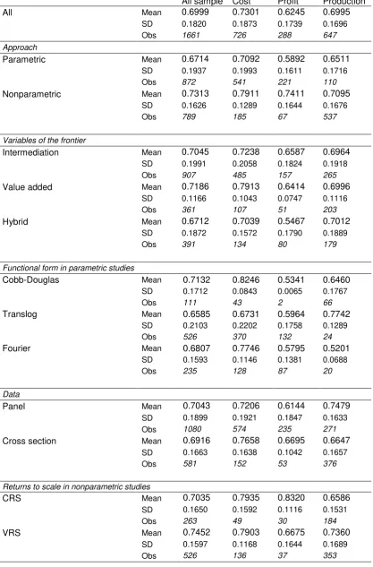
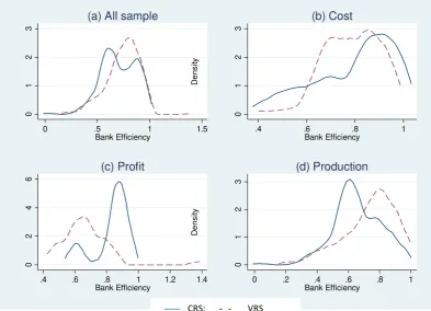
A synthesis of the collected estimates is reported in table 2, where different sub-samples of scores have been considered according to the approach used in estimations (parametric or nonparametric), the approach followed in selecting the variable for the frontiers (intermediation, value added or hybrid approaches), the structure of data (panel or cross-section), the functional form of the frontier (Cobb-Douglas, translog or Fourier) and, finally, on the basis of the hypotheses regarding returns to scale (constant or variable).

Overall, the sample of 1,661 observations yields an average efficiency of 0.69. Some differences emerge by efficiency type: the average of the 726 cost-efficiency scores is 0.73, while it is 0.62 for 288 observations based on profit frontiers. In the case of the 647 observations of efficiency in production, the average is 0.69. data also highlight that the overall mean of the 872 observations from parametric studies is always lower than that of the 789 observations of nonparametric papers: the difference in mean is 0.0599 (0.7313-0.6714) and is statistically significant.4

Differences between the efficiency of nonparametric and parametric studies remain positive and significant, whatever type of efficiency we refer to (cost, profit or production). Again, there are 907 observations referring to studies using the intermediation approach, more than 50% of the entire sample, while the dataset includes 361 observations from studies using the value added approach. Between these two extremes, there is the hybrid approach, which differs in that researchers consider deposits either as input or output. The hybrid approach is made up of 391 observations. The difference in means is only high when

(14)

13

considering the cost-frontier where the production approach yields a higher (0.7913) average efficiency than the intermediation (0.7238) and the hybrid (0.7039) choices. With regards the structure of data used in primary studies, the analysis shows that about two-thirds of the observations come from estimations obtained from panel data and the other one-third refers to cross-section data. What clearly emerges is that there is no difference in means when considering the entire sample of observations, while cost and profit efficiency scores are higher, on average, when using cross-section instead of panel data. The opposite holds for the other measures of efficiency. Furthermore, in the sample of parametric studies, another difference is that few (111 in the full sample) observations refer to a Cobb-Douglas specification of the frontier, while the majority use more flexible functional forms (526 adopt a translog frontier and 235 a Fourier one). While Cobb-Douglas specifications yield a higher level of efficiency when studying cost efficiency (0.8246 compared with 0.6731 from translog and 0.7746 from Fourier), the translog form applied to profit frontier yields a higher value of efficiency (0.5964 compared with 0.5341 from Cobb-Douglas and 0.5795 from Fourier). Finally, an interesting pattern is observed when referring to the hypothesis of returns to scale of nonparametric-studies. Overall, the assumption of VRS translates to an average level of efficiency (0.7452) which is higher than that (0.7035) associated with the observations using the hypothesis of CRS. However. results differ according to the frontier. For instance, when considering profit frontiers, we find that the average level of efficiency obtained in the primary studies using CRS is 0.8320, that is to say a much higher value than that (0.6675) associated with the studies based on VRS.

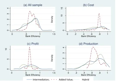
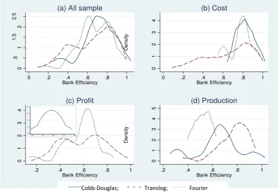
A lesson learnt from this discussion is that the study-design of primary papers plays an important role in determining differences in the means of banking efficiency scores. In addition, the heterogeneity in banking efficiency literature is confirmed by figures 3-7, which display the distribution of the estimated scores by group. The exposition of results follows the same strategy in each figure. For instance, panel A of figure 3 refers to the full sample and presents the efficiency scores obtained from parametric and nonparametric methods. It is clear that the density functions have different shapes and forms. The likely effect of choosing to estimate banking efficiency through a parametric or a nonparametric method is even more evident when splitting the sample by cost efficiency (panel b), profit efficiency (panel c) and efficiency in production (panel d). The distributions are more uneven when comparing the intermediation, value added and the hybrid methods (figure 4). The same applies for the remaining cases, except for some overlapping of the distribution of cost-efficiency reported in panel data and cross section studies (figure 5, panel b).5

(15)

[image:15.595.90.508.122.756.2]

14

Table 2 Average, standard deviation and number of observations in bank efficiency literature by group

All sample Cost Profit Production

All Mean 0.6999 0.7301 0.6245 0.6995

SD 0.1820 0.1873 0.1739 0.1696 Obs 1661 726 288 647 Approach

Parametric Mean 0.6714 0.7092 0.5892 0.6511

SD 0.1937 0.1993 0.1611 0.1716

Obs 872 541 221 110

Nonparametric Mean 0.7313 0.7911 0.7411 0.7095

SD 0.1626 0.1289 0.1644 0.1676

Obs 789 185 67 537

Variables of the frontier

Intermediation Mean 0.7045 0.7238 0.6587 0.6964

SD 0.1991 0.2058 0.1824 0.1918

Obs 907 485 157 265

Value added Mean 0.7186 0.7913 0.6414 0.6996

SD 0.1166 0.1043 0.0747 0.1116

Obs 361 107 51 203

Hybrid Mean 0.6712 0.7039 0.5467 0.7012

SD 0.1872 0.1572 0.1790 0.1889

Obs 391 134 80 179

Functional form in parametric studies

Cobb-Douglas Mean 0.7132 0.8246 0.5341 0.6460

SD 0.1712 0.0843 0.0065 0.1767

Obs 111 43 2 66

Translog Mean 0.6585 0.6731 0.5964 0.7742

SD 0.2103 0.2202 0.1758 0.1289

Obs 526 370 132 24

Fourier Mean 0.6807 0.7746 0.5795 0.5201

SD 0.1593 0.1146 0.1381 0.0688

Obs 235 128 87 20

Data

Panel Mean 0.7043 0.7206 0.6144 0.7479

SD 0.1899 0.1921 0.1847 0.1633 Obs 1080 574 235 271

Cross section Mean 0.6916 0.7658 0.6695 0.6647

SD 0.1663 0.1638 0.1042 0.1657

Obs 581 152 53 376

Returns to scale in nonparametric studies

CRS Mean 0.7035 0.7935 0.8320 0.6586

SD 0.1650 0.1592 0.1116 0.1531

Obs 263 49 30 184

VRS Mean 0.7452 0.7903 0.6675 0.7360

SD 0.1597 0.1168 0.1644 0.1689

(16)

15 0 .5 1 1 .5 2 2 .5

0 .5 1 1.5

Bank Efficiency

(a) All sample

0 1 2 3 D e n s ity

0 .2 .4 .6 .8 1

Bank Efficiency (b) Cost 0 .5 1 1 .5 2 2 .5

0 .5 1 1.5

Bank Efficiency (c) Profit 0 .5 1 1 .5 2 2 .5 D e n s ity

0 .2 .4 .6 .8 1

Bank Efficiency

(d) Production

[image:16.595.104.500.110.376.2]

Parametric; Nonparametric

Figure 3 Distribution of banking efficiency by estimating method (parametric and nonparametric)

Figure 4 Distribution of banking efficiency by variables approach (intermediation, value added and hybrid)

0

1

2

3

4

0 .5 1 1.5

Bank Efficiency

(a) All sample

0 5 10 15 D e n s ity

0 .2 .4 .6 .8 1

Bank Efficiency

(b) Cost

0

5

10

0 .5 1 1.5

Bank Efficiency (c) Profit 0 1 2 3 4 D e n s ity

0 .2 .4 .6 .8 1

Bank Efficiency

(d) Production

[image:16.595.106.505.456.734.2]

(17)

16 0 .5 1 1 .5 2 2 .5

0 .5 1 1.5

Bank Efficiency

(a) All sample

0 1 2 3 D e n s ity

0 .2 .4 .6 .8 1

Bank Efficiency (b) Cost 0 1 2 3 4 5

0 .5 1 1.5

Bank Efficiency (c) Profit 0 1 2 3 4 D e n s ity

0 .2 .4 .6 .8 1

Bank Efficiency

(d) Production

Panel; Cross section

0 .5 1 1 .5 2 2 .5

0 .2 .4 .6 .8 1

Bank Efficiency

(a) All sample

0 1 2 3 4 D e n s ity

0 .2 .4 .6 .8 1

Bank Efficiency (b) Cost 0 1 2 3 4

.2 .4 .6 .8 1

Bank Efficiency (c) Profit 0 1 2 3 4 5 D e n s ity

.2 .4 .6 .8 1

Bank Efficiency

(d) Production

Cobb-Douglas; Translog; Fourier

20

30

40

50

60

[image:17.595.107.505.113.384.2]

.525 .53 .535 .54 .545

Figure 5 Distribution of banking efficiency by data type (panel and cross section)

[image:17.595.107.506.461.735.2]

(18)

17

0

1

2

3

0 .5 1 1.5

Bank Efficiency (a) All sample

0

1

2

3

D

e

n

s

it

y

.4 .6 .8 1

Bank Efficiency (b) Cost

0

2

4

6

.4 .6 .8 1 1.2 1.4

Bank Efficiency (c) Profit

0

1

2

3

D

e

n

s

it

y

0 .2 .4 .6 .8 1

Bank Efficiency (d) Production

[image:18.595.110.504.113.397.2]

CRS; VRS

Figure 7 Distribution of banking efficiency by return to scale (CRS and VRS)

6. Meta-analysis regression and results

6.1 The empirical setting

The descriptive evidence indicates that there are relevant differences in means and in the efficiency distributions when grouping observations by different criteria. Given this, providing a systematic explanation of the variability of efficiency becomes an important issue to be addressed on econometric grounds. This section focuses on meta-regression analysis carried out to explain heterogeneity in banking efficiency scores. We proceed by (i) introducing the estimator used in the empirical analysis and presenting the econometric specification of the meta-regression and by (ii) discussing the results.

There are two main issues to be addressed in our empirical analysis. The first regards heteroschedasticity, while the second relates to publication bias.

(19)

18

al., 1997). If this regression yields significant results, then there is evidence of publication bias in the meta-data set which must be controlled for in the meta-regression.

This said , in order to provide answers to the research questions raised throughout the paper, we refer to the following equation:

i i S       



j j j 0 1

i β X

E [1]

where the dependent variable Ei is the i-th efficiency score. Xj is comprised of the explicative

variables that summarize various model characteristics of the primary studies. Si is a measure of variability of Ei and enters into the meta-regression to control for publication bias as proposed by Egger et. al. (1997) and applied by Bumann et al. (2013), Cipollina and Salvatici (2007), Feld et al. (2013) and Stanley (2008). ε is the error of the model, which is clearly heteroschedastic because the variance of individual estimates changes in the sample and the estimates are not independent within the same study (Stanley, 2008). This issue is addressed by weighting the observation through a measure S of the variability of each observation:

i i i i i i i i e X S E e S S S        



j * j * 1 0 * j j j 1 0 i β X β 1 E     [2]

where the disturbance e S is corrected for heteroschedasticity- The test for publication

bias will be carried out on the constant 0, as in Cipollina and Salvatici (2007), Doucouliagos

and Stanley (2009), Fed et al. (2013) and Stanley (2008).

The method to be used in estimating eq. [2] may be a fixed-effects or a random-effects model. While both methods provide results which are robust to publication bias (Stanley 2008), they differ in terms of their treatment of heterogeneity. In particular, a fixed-effects meta-regression assumes that all the heterogeneity can be explained by the covariates and leads to excessive type I errors when there is residual, or unexplained, heterogeneity (Harbord and Higgins, 2008; Higgins and Thompson, 2004; Thompson and Sharp, 1999). Instead, a random-effects meta-regression allows for such residual heterogeneity (the between-study variance not explained by the covariates) and therefore extends the fixed-effects model. Formally, under the random-fixed-effects framework, eq. [2] becomes:

i i i i

i S X u e

E   



 

j * j * 1 0

*   β [3]

where ei ~ N(θi , σ2i) is the disturbance and ui ~ N(θi , τ 2) is the fixed-effect. The parameter τ2 is the between-study variance, which must be estimated from the data as in Harbord and

Higgins (2008).6

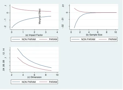
The right-hand side of eq. [3] includes Xj which relates to the firm observed characteristics used to explain the variability in banks’ efficiency and we have identified on

6_{Technically, REML first estimates the between-study variance,}

(20)

19

the basis of a systematic comparison of original papers. In selecting the moderator variables, we bear in mind the fact that the focus is to verify whether the methodology choices followed in primary works matter in determining the mean efficiency of the banking industry. The explanatory variables follow.

The first distinguishing element to be considered relates to the approach used to estimate the frontier. We made a broad distinction between papers using a parametric method and papers following a nonparametric approach. To this end, the dummy variable used is Parametric (PA) which is equal to unity for the first group of studies and zero for the others. As we have already said (cfr. § 5), scholars use deposits as inputs or outputs in banking literature. In this respect, we include the dummies Intermediation (INT) and Value added (Y), which are unity when efficiency scores are derived from primary-studies using the intermediation or the value added approach (the controlling group comprises the point-observations from papers using the hybrid approach, HY). Furthermore, the entire sample comprises three types of efficiency, cost, profit and production efficiency. To control for this, we include two dummies, Cost (CE) and Profit (PE), with the value 1 if the efficiency score refers to cost or profit efficiencies (the controlling group is the efficiency obtained a production frontier).

The literature on Meta-Regression helps to select the other controlling variables. A element which should be considered is the time period analyzed. Increasing regulation is expected to gradually lead to improvements in how banks work, other things being equal. This time-effect is meant to be gauged by the dummies Y2000-2004 and Y2005-2009, which are equal

(21)

20 6.2 Econometric Results

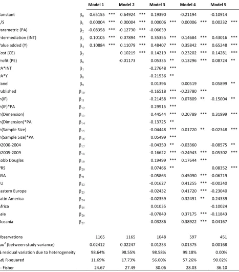
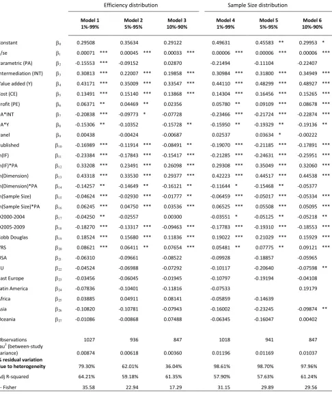
In presenting the results, we start from a basic regression which includes just the dummies relating to the methodological choices made when performing an estimation of banks_’ efficiency. The underlying idea is to test the robustness of results (sign, magnitude and significance) when moving from basic to extended regressions. In table 3, Model 1 considers just the variables Parametric, Intermediation and Value added. Model 2 controls for the type of efficiency effect and, to this end, adds the variables Cost and Profit to Model 1. Model 3 is the expanded version of our meta-regression, introducing the interacting terms PA*Y and PA*INT and considering all the other moderator variables in order to better identify the origin of the heterogeneity in banking efficiency, as already defined. Model 4 and 5 limit the analysis to the sub-samples of studies belonging to the class of parametric and nonparametric, respectively.7_{Table 4 displays the results obtained from a sensitivity analysis which was}

carried out to test whether the evidence is robust to the exclusion of 1%, 5% and 10% tails of the efficiency and sample size distributions.8

Before the results are presented, it is worthwhile commenting on some diagnostics. The main evidence regards ˆ0, the parameter used as a test for publication bias: ˆ0 is

significant in Model 1 and 2 and not in Models 3, 4 and 5 of table 3. Findings in table 3 indicate that there is no evidence of publication bias when covariates enter into regressions to explain the heterogeneity in efficiency. The same applies after excluding the tails of the key variable of our study, that is to say the efficiency distribution (table 4). Furthermore, we present some statistics at the bottom of each table that we retrieved from the Stata-command “metareg”

developed by Harbord and Higgins (2008). As can be seen, the proportion of the residual variance that is attributable to between-study heterogeneity is very high. In Model 3, it is 98.58%. Again, in the same regression, the proportion of between variance explained by the covariates is 56%, the measure of within-study sampling variability. Finally, the joint-significance of moderators is high in each model.

In order to ensure clarity in the presentation of results, the discussion is divided into two sub-sections. The first devotes attention to the role of estimating methods and approaches in the choice of variables, while the second sub-section looks at the effects exerted by the other variables included in the meta-regression.

6.2.1 The roles of the estimating method and variable approaches

The first finding to be discussed regards the role of using parametric or nonparametric methods. This issue is important because the majority of parametric studies in our sample use SFA and, similarly, almost all nonparametric studies are based on DEA, which is expected to determine higher efficiency indexes than stochastic models do (Ekanayake and Jayasuriya, 1987). According to our estimates, parametric techniques generate significantly lower

7_{Splitting the sample should allow better evaluation of the role of specific methodological choices. For}

instance, this is the case of the dummy Cobb-Douglas: in model 4 the “zeros” only refer to functional forms other than Cobb-Douglas and not to point-observations from nonparametric studies, as in Model 3. The same applies for the dummy VRS. Even though assumptions on return to scale are possible whatever the method, many parametric studies do not report which return to scale they use and there is no way to understand the assumption. While the procedure followed in Models 4 and 5 is more appropriate compared with Model 3, it is interesting to point out that the results do not change moving from Model 3 to Model 4 or to Model 5 (see table 3).

8

(22)

21

efficiency scores than nonparametric models do: the coefficient associated with the dummy Parametric is negative and highly significant in Models 1 and 2, indicating that, other things being fixed, the efficiency scores are lower for parametric than for nonparametric techniques. This is in line with the movement of the erratic component as depicted in the hypothetical case of bank A in figure 1: in reviewing the banking literature, we find that the random noise is high and positive and, thus, that the efficiency scores from parametric procedures are systematically lower than those obtained from nonparametric ones (cfr. figure 1). This finding is confirmed after controlling for the approach used in selecting the variables, as can be seen from Model 3 (see the results displayed in table 5 below). It is also worth pointing out that the parametric effect in the other MA applications is found to be neutral with respect to the counterpart, as documented by the inconclusive evidence provided by Thiam et al. (2001) for agriculture in developing countries, Coelli and Nguyen (2009) for hospitals, Brons et al. (2005) for transport and Kolawole (2009) for Nigerian agriculture. Conversely, some similarity with our evidence is found in Bravo-Ureta et al (2007) with regard the agricultural efficiency in developed and developing economies and in Odeck and Bråthen (2009) for efficiency in seaports.

We also show that the approach (value added, intermediation or hybrid) followed in choosing inputs and outputs of the frontier is relevant in the evaluation of banking efficiency. Estimations of Models 1 and 2 indicate that the dummy variable Intermediation is always positive, suggesting that studies based on the intermediation approach provide, all being equal, efficiency scores which are higher that those generated by the hybrid approach. The same applies for the value added approach. The order between the effect exerted by the intermediation and the value added approaches depends upon the model we refer to. When considering Model 1, both value added and intermediation approaches over-perform compared with the hybrid and share the same effect (ˆ₃ 0.1;ˆ₄ 0.11). In moving to Model

2, we find that, on average, the value added approach yields the highest level of efficiency, followed by the intermediation and the hybrid approaches (ˆ4 0.11and ˆ3 0.078). The

main conclusions to be drawn are that the hybrid approach generates low levels of efficiency, followed by the intermediation approach. The highest average level of banking efficiency is yielded by papers based on the value added approach.

The discussion presented so far concerns the effects on the efficiency due to a particular methodological choice rather than another, excluding the possible effects relating to choices that combine the different methods. For instance, it is fruitful to test whether efficiency scores differ when combining the parametric and variable approaches (intermediation, value added or hybrid). Similarly, it appears important to understand whether efficiency differs when using parametric or nonparametric methods, provided that the variables of the frontier are chosen according to one of the three approaches. These issues may be addressed by augmenting the meta-regression with the interacting terms PA*INT and PA*Y. Compared with the basic model 1 of table 3, the regression to be estimated now becomes:









i i

j j i i u Y PA INT PA X Y INT PA S E j                    



* * ₈ 7 * 4 3 2 * 1 0 * [4]

(23)

23

By using results of Model 3 displayed in table 3, in table 5 we report the differences in efficiency obtained when using one variable approach over another, within the class of parametric or nonparametric studies (panel A). The findings confirm the role played by the approach to be followed when selecting the variables of the frontier. The intermediation and the value added approaches yield higher efficiency scores than the hybrid approach does. This holds true in both parametric and nonparametric estimates, although the difference is significant in the latter group. Indeed, when comparing the average level of efficiency resulting from the intermediation and the hybrid approaches, we find a difference of 0.138 in parametric studies and of 0.35 in nonparametric methods. Similarly, while the difference between the value added and the hybrid approaches is 0.2 in parametric studies, it becomes 0.48 in the nonparametric group. The conclusion we can draw is that use of the hybrid approach generates a lower level of efficiency scores than the intermediation and the value added approaches, whatever the method chosen to estimate the frontier. There are also some differences between the intermediation and the value added approaches: on average, the first generates lower levels of efficiency than the second, in both the parametric and nonparametric classes. The difference is low (0.069) in parametric studies and increases to -0.13 for nonparametric methods (table 5, panel A).

Another finding provided by the estimations of Model 3 regards the evaluation of choosing a parametric instead of a nonparametric method, assuming that the approach taken to select the variables is fixed (table 5, panel B). What clearly emerges is similar to what is found in Models 1 and 2. While Models 1 and 2 refer to an overall effect of parametric versus nonparametric methods, the use of Model 3 disaggregates the evidence by intermediation, value added and hybrid approaches. According to our computations, parametric studies yield, on average, an efficiency level of -0.21 less than nonparametric studies when using the intermediation approach. The difference becomes -0.27 when the value added approach is taken into account. No difference exists within the hybrid approach: indeed the coefficient ₂

(25)

[image:25.595.67.535.89.621.2]

24

Table 3 Meta-regression of banking efficiency scores. REML estimations.

Model 1 Model 2 Model 3 Model 4 Model 5

Constant  0.65155 *** 0.64924 *** 0.19390 -0.21194 -0.10914

1/S _ 0.00004 *** 0.00004 *** 0.00006 *** 0.00006 *** 0.00232 ***

Parametric (PA)  -0.08358 *** -0.12730 *** -0.06639

Intermediation (INT) _ 0.10105 *** 0.07894 *** 0.35355 *** 0.14684 *** 0.43016 ***

Value added (Y)  0.10884 *** 0.11079 *** 0.48407 *** 0.35842 *** 0.65248 ***

Cost (CE) _ 0.10219 *** 0.14219 *** 0.23202 *** 0.14281 ***

Profit (PE)  -0.01173 0.05335 ** 0.13296 *** 0.08724 **

PA*INT _ -0.27648 ***

PA*Y  -0.21536 **

Panel _ 0.01396 0.00519 0.05899 **

Published  -0.16518 *** -0.23780 ***

ln(IF) _ -0.21458 *** 0.07809 ** -0.15004 **

ln(IF)*PA  0.29915 ***

ln(Dimension) _ 0.44544 *** 0.20789 *** 0.31999 ***

ln(Dimension)*PA  -0.13725 **

ln(Sample Size) _ -0.04448 *** 0.01720 ** -0.02348 ***

ln(Sample Size)*PA  0.05499 ***

D2000-2004 _ -0.04350 ** -0.03360 -0.08575 **

D2005-2009  -0.16622 *** -0.24943 *** 0.05302 ***

Cobb Douglas _ 0.19499 *** 0.17644 ***

VRS  0.07466 ** 0.08352 ***

USA _ -0.05863 0.45090 *** -0.06719

EU  -0.01627 0.41255 *** -0.00240

Eastern Europe _ -0.02432 0.41720 *** -0.23040

Latin America  -0.02359 0.32491 ** 0.24339

Africa _ 0.01035 -0.10024

Asia  -0.07840 0.37175 *** -0.11843

Oceania _ 0.03286 0.38922 *** 0.04167

Observations 1165 1165 1048 597 451

tau2 (between-study variance) 0.02412 0.02247 0.01233 0.01375 0.00168

% residual variation due to heterogeneity 98.64% 98.55% 98.58% 99.18% 0.00%

Adj R-squared 11.69% 17.73% 56.00% 57.26% 90.02%

(26)

[image:26.595.63.550.104.681.2]

25

Table 4 Meta-regression of banking efficiency scores. A sensitivity analysis. REML estimations.

Efficiency distribution Sample Size distribution

Model 1 1%-99%

Model 2 5%-95%

Model 3 10%-90%

Model 4 1%-99%

Model 5 5%-95%

Model 6 10%-90%

Constant  0.29508 0.35634 0.29122 0.49631 0.45583 ** 0.29953 *

1/se  0.00071 *** 0.00045 *** 0.00033 *** 0.00006 *** 0.00006 *** 0.00006 ***

Parametric (PA)  -0.15553 *** -0.09152 0.02870 -0.21494 -0.11104 -0.22407

Intermediation (INT)  0.30813 *** 0.22007 *** 0.19858 *** 0.30984 *** 0.31800 *** 0.34949 ***

Value added (Y)  0.43171 *** 0.35009 *** 0.33547 *** 0.44110 *** 0.48299 *** 0.48927 ***

Cost (CE)  0.13491 *** 0.15140 *** 0.13868 *** 0.14304 *** 0.16456 *** 0.15265 ***

Profit (PE)  0.06371 ** 0.04469 ** 0.02356 0.05780 ** 0.09109 *** 0.08678 ***

PA*INT  -0.20838 *** -0.09773 * -0.07728 -0.23466 *** -0.21724 *** -0.22874 ***

PA*Y  -0.15306 ** -0.10352 -0.15728 ** -0.15950 ** -0.19329 ** -0.19136 **

Panel  0.00438 -0.00424 -0.00687 0.02537 0.03634 * -0.00222

Published  -0.16989 *** -0.11914 *** -0.08491 ** -0.19070 *** -0.21185 *** -0.17891 ***

ln(IF)  -0.23384 *** -0.17843 *** -0.15417 *** -0.21285 *** -0.24631 *** -0.25951 ***

ln(IF)*PA  0.33208 *** 0.23491 *** 0.26098 *** 0.29308 *** 0.35049 *** 0.32060 ***

ln(Dimension)  0.43318 *** 0.33530 *** 0.29377 *** 0.42223 *** 0.44517 *** 0.44538 ***

ln(Dimension)*PA  -0.14257 ** -0.14649 ** -0.16121 ** -0.11644 * -0.15468 ** -0.05377

ln(Sample Size)  -0.04624 *** -0.02930 *** -0.01777 ** -0.06459 *** -0.05017 *** -0.05334 ***

ln(Sample Size)*PA  0.06245 *** 0.04750 *** 0.03536 *** 0.06525 *** 0.05508 *** 0.05095 ***

D2000-2004  -0.04250 ** -0.02557 0.00300 -0.03551 * -0.05125 ** -0.05218 **

D2005-2009  -0.18270 *** -0.13317 *** -0.09463 *** -0.17783 *** -0.19310 *** -0.18553 ***

Cobb Douglas  0.18524 *** 0.15680 *** 0.11836 *** 0.19022 *** 0.21029 *** 0.15929 ***

VRS  0.08621 *** 0.06411 ** 0.07654 *** 0.05481 ** 0.07775 ** 0.09121 ***

USA  -0.06310 -0.09661 -0.08522 -0.09928 -0.18857 -0.05965

EU  -0.04524 -0.06988 -0.07292 -0.10117 -0.20640 -0.07598 **

East Europe  -0.03456 -0.06045 -0.01945 -0.10797 -0.19194 -0.04108

Latin America  -0.07836 -0.10401 -0.11816 -0.07533 0.19179

Africa  0.03885 0.04911 0.08141 -0.05859 -0.14639

Asia  -0.10820 -0.10781 -0.07943 -0.16002 -0.23245 -0.09874 **

Oceania  -0.01086 -0.00868 0.07488 -0.06345 -0.16047 0.00402

Observations 1027 936 847 1018 941 847

tau2 (between-study

variance) 0.00874 0.00618 0.00360 0.01196 0.01169 0.01037

% residual variation

due to heterogeneity 79.30% 62.01% 36.04% 98.61% 98.70% 97.96%

Adj R-squared 64.21% 59.18% 61.35% 57.90% 57.63% 61.24%