Dynamic Programming for Linear-Time Incremental Parsing
Liang Huang
USC Information Sciences Institute 4676 Admiralty Way, Suite 1001
Marina del Rey, CA 90292 [email protected]
Kenji Sagae
USC Institute for Creative Technologies 13274 Fiji Way
Marina del Rey, CA 90292 [email protected]
Abstract
Incremental parsing techniques such as shift-reduce have gained popularity thanks to their efficiency, but there remains a major problem: the search is greedy and only explores a tiny fraction of the whole space (even with beam search) as op-posed to dynamic programming. We show that, surprisingly, dynamic programming is in fact possible for many shift-reduce parsers, by merging “equivalent” stacks based on feature values. Empirically, our algorithm yields up to a five-fold speedup over a state-of-the-art shift-reduce depen-dency parser with no loss in accuracy. Bet-ter search also leads to betBet-ter learning, and our final parser outperforms all previously reported dependency parsers for English and Chinese, yet is much faster.
1 Introduction
In terms of search strategy, most parsing al-gorithms in current use for data-driven parsing can be divided into two broad categories: dy-namic programming which includes the domi-nant CKY algorithm, and greedy search which in-cludes most incremental parsing methods such as shift-reduce.1 Both have pros and cons: the for-mer performs an exact search (in cubic time) over an exponentially large space, while the latter is much faster (in linear-time) and is psycholinguis-tically motivated (Frazier and Rayner, 1982), but its greedy nature may suffer from severe search er-rors, as it only explores a tiny fraction of the whole space even with a beam.
Can we combine the advantages of both ap-proaches, that is, construct an incremental parser
1McDonald et al. (2005b) is a notable exception: the MST algorithm is exact search but not dynamic programming.
that runs in (almost) linear-time, yet searches over a huge space with dynamic programming?
Theoretically, the answer is negative, as Lee (2002) shows that context-free parsing can be used to compute matrix multiplication, where sub-cubic algorithms are largely impractical.
We instead propose a dynamic programming al-ogorithm for shift-reduce parsing which runs in polynomial time in theory, but linear-time (with beam search) in practice. The key idea is to merge equivalent stacks according to feature functions, inspired by Earley parsing (Earley, 1970; Stolcke, 1995) and generalized LR parsing (Tomita, 1991). However, our formalism is more flexible and our algorithm more practical. Specifically, we make the following contributions:
• theoretically, we show that for a large class of modern shift-reduce parsers, dynamic pro-gramming is in fact possible and runs in poly-nomial time as long as the feature functions are bounded and monotonic (which almost al-ways holds in practice);
• practically, dynamic programming is up to five times faster (with the same accuracy) as conventional beam-search on top of a state-of-the-art shift-reduce dependency parser;
• as a by-product, dynamic programming can output a forest encoding exponentially many trees, out of which we can draw better and longerk-best lists than beam search can;
• finally, better and faster search also leads to better and faster learning. Our final parser achieves the best (unlabeled) accuracies that we are aware of in both English and Chi-nese among dependency parsers trained on the Penn Treebanks. Being linear-time, it is also much faster than most other parsers, even with a pure Python implementation.
input: w0. . . wn−1
axiom 0 :h0, ǫi:0
sh ℓ:hj, Si:c
ℓ+ 1 :hj+ 1, S|wji:c+ξ j < n
re x
ℓ:hj, S|s1|s0i:c
ℓ+ 1 :hj, S|s1xs0i:c+λ
re y
ℓ:hj, S|s1|s0i:c
ℓ+ 1 :hj, S|s1ys0i:c+ρ
goal 2n−1 :hn, s0i:c
whereℓis the step,cis the cost, and the shift costξ and reduce costsλandρare:
ξ = w·fsh(j, S) (1)
λ = w·frex(j, S|s1|s0) (2)
[image:2.595.70.275.62.236.2]ρ = w·frey(j, S|s1|s0) (3)
Figure 1: Deductive system of vanilla shift-reduce.
For convenience of presentation and experimen-tation, we will focus on shift-reduce parsing for dependency structures in the remainder of this pa-per, though our formalism and algorithm can also be applied to phrase-structure parsing.
2 Shift-Reduce Parsing
2.1 Vanilla Shift-Reduce
Shift-reduce parsing performs a left-to-right scan of the input sentence, and at each step, choose one of the two actions: either shift the current word onto the stack, or reduce the top two (or more) items at the end of the stack (Aho and Ullman, 1972). To adapt it to dependency parsing, we split the reduce action into two cases,re
xandrey,
de-pending on which one of the two items becomes the head after reduction. This procedure is known as “arc-standard” (Nivre, 2004), and has been en-gineered to achieve state-of-the-art parsing accu-racy in Huang et al. (2009), which is also the ref-erence parser in our experiments.2
More formally, we describe a parser configura-tion by a state hj, Si where S is a stack of trees
s0, s1, ... where s0 is the top tree, and j is the
2There is another popular variant, “arc-eager” (Nivre, 2004; Zhang and Clark, 2008), which is more complicated and less similar to the classical shift-reduce algorithm.
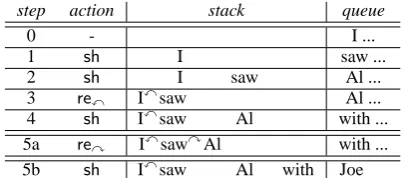
input: “I saw Al with Joe”
step action stack queue
0 - I ...
1 sh I saw ...
2 sh I saw Al ...
3 rex Ixsaw Al ...
4 sh Ixsaw Al with ...
5a re
y IxsawyAl with ...
5b sh Ixsaw Al with Joe
Figure 2: A trace of vanilla shift-reduce. After step (4), the parser branches off into (5a) or (5b).
queue head position (current word q0 is wj). At
each step, we choose one of the three actions:
1. sh: move the head of queue,wj, onto stackS
as a singleton tree;
2. re
x: combine the top two trees on the stack,
s0ands1, and replace them with trees1xs0.
3. re
y: combine the top two trees on the stack,
s0ands1, and replace them with trees1ys0.
Note that the shorthand notation txt′ denotes a
new tree by “attaching treet′as the leftmost child
of the root of treet”. This procedure can be sum-marized as a deductive system in Figure 1. States are organized according to step ℓ, which denotes the number of actions accumulated. The parser runs in linear-time as there are exactly2n−1steps for a sentence ofnwords.
As an example, consider the sentence “I saw Al with Joe” in Figure 2. At step (4), we face a shift-reduce conflict: either combine “saw” and “Al” in are
yaction (5a), or shift “with” (5b). To resolve
this conflict, there is a costcassociated with each state so that we can pick the best one (or few, with a beam) at each step. Costs are accumulated in each step: as shown in Figure 1, actionssh,re
x,
and re
y have their respective costs ξ, λ, and ρ,
which are dot-products of the weightswand
fea-tures extracted from the state and the action.
2.2 Features
[image:2.595.315.518.79.168.2]of two atomic features s0.w andq0.t, capturing
the root word of the top tree s0 on the stack, and
the part-of-speech tag of the current head wordq0
on the queue. See Tab. 1(a) for the list of feature templates used in the full model. Feature templates are instantiated for a specific state. For example, at step (4) in Fig. 2, the above templatef100will
gen-erate a feature instance
(s0.w=Al)◦(q0.t=IN).
More formally, we denotefto be the feature func-tion, such that f(j, S) returns a vector of feature
instances for statehj, Si. To decide which action is the best for the current state, we perform a three-way classification based on f(j, S), and to do so,
we further conjoin these feature instances with the action, producing action-conjoined instances like
(s0.w=Al)◦(q0.t=IN)◦(action =sh).
We denotefsh(j, S),fre
x(j, S), andfrey(j, S) to
be the conjoined feature instances, whose dot-products with the weight vector decide the best ac-tion (see Eqs. (1-3) in Fig. 1).
2.3 Beam Search and Early Update
To improve on strictly greedy search, shift-reduce parsing is often enhanced with beam search (Zhang and Clark, 2008), where bstates develop in parallel. At each step we extend the states in the current beam by applying one of the three ac-tions, and then choose the best b resulting states for the next step. Our dynamic programming algo-rithm also runs on top of beam search in practice.
To train the model, we use the averaged percep-tron algorithm (Collins, 2002). Following Collins and Roark (2004) we also use the “early-update” strategy, where an update happens whenever the gold-standard action-sequence falls off the beam, with the rest of the sequence neglected.3The intu-ition behind this strategy is that later mistakes are often caused by previous ones, and are irrelevant when the parser is on the wrong track. Dynamic programming turns out to be a great fit for early updating (see Section 4.3 for details).
3 Dynamic Programming (DP)
3.1 Merging Equivalent States
The key observation for dynamic programming is to merge “equivalent states” in the same beam
3As a special case, for the deterministic mode (b=1), up-dates always co-occur with the first mistake made.
(a) Features Templatesf(j, S) qi=wj+i
(1) s0.w s0.t s0.w◦s0.t
s1.w s1.t s1.w◦s1.t
q0.w q0.t q0.w◦q0.t
(2) s0.w◦s1.w s0.t◦s1.t
s0.t◦q0.t s0.w◦s0.t◦s1.t
s0.t◦s1.w◦s1.t s0.w◦s1.w◦s1.t
s0.w◦s0.t◦s1.w s0.w◦s0.t◦s1◦s1.t
(3) s0.t◦q0.t◦q1.t s1.t◦s0.t◦q0.t
s0.w◦q0.t◦q1.t s1.t◦s0.w◦q0.t
(4) s1.t◦s1.lc.t◦s0.t s1.t◦s1.rc.t◦s0.t
s1.t◦s0.t◦s0.rc.t s1.t◦s1.lc.t◦s0
s1.t◦s1.rc.t◦s0.w s1.t◦s0.w◦s0.lc.t
(5) s2.t◦s1.t◦s0.t
(b) ←stack queue→
... s2
...
s1
s1.lc
...
... s1.rc
...
s0
s0.lc
...
... s0.rc
...
q0 q1 ...
(c) Kernel features for DP
ef(j, S) = (j,f2(s2),f1(s1),f0(s0)) f2(s2) s2.t
f1(s1) s1.w s1.t s1.lc.t s1.rc.t f0(s0) s0.w s0.t s0.lc.t s0.rc.t
[image:3.595.306.520.60.361.2]j q0.w q0.t q1.t
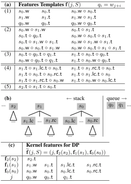
Table 1: (a) feature templates used in this work, adapted from Huang et al. (2009).x.wandx.t
de-notes the root word and POS tag of tree (or word) x. andx.lcandx.rcdenotex’s left- and rightmost child. (b) feature window. (c) kernel features.
(i.e., same step) if they have the same feature values, because they will have the same costs as shown in the deductive system in Figure 1. Thus we can define two stateshj, Si andhj′, S′i to be equivalent, notatedhj, Si ∼ hj′, S′i, iff.
j=j′ and f(j, S) =f(j′, S′). (4)
Note that j = j′ is also needed because the
queue head position j determines which word to shift next. In practice, however, a small subset of atomic features will be enough to determine the whole feature vector, which we call kernel
fea-turesef(j, S), defined as the smallest set of atomic
templates such that
ef(j, S) =ef(j′, S′)⇒ hj, Si ∼ hj′, S′i.
For example, the full list of 28 feature templates in Table 1(a) can be determined by just 12 atomic features in Table 1(c), which just look at the root words and tags of the top two trees on stack, as well as the tags of their left- and rightmost chil-dren, plus the root tag of the third trees2, and
state form ℓ:hi, j, sd...s0i:(c, v, π) ℓ: step;c,v: prefix and inside costs;π: predictor states
equivalence ℓ:hi, j, sd...s0i ∼ℓ:hi, j, s′d...s′0i iff. ef(j, sd...s0) =fe(j, s′d...s′0)
ordering ℓ: : (c, v, )≺ℓ: : (c′, v′, ) iff.c < c′or (c=c′ andv < v′).
axiom (p0) 0 :h0, 0, ǫi: (0,0,∅)
sh
statep:
ℓ:h , j, sd...s0i: (c, , )
ℓ+ 1 :hj, j+ 1, sd−1...s0, wji: (c+ξ, 0, {p}) j < n
re x
statep:
:hk, i, s′d...s′0i: (c′, v′, π′)
stateq:
ℓ:hi, j, sd...s0i: ( , v, π)
ℓ+ 1 :hk, j, s′d...s′1, s′0xs0i: (c′+v+δ, v′+v+δ, π′)
p∈π
goal 2n−1 :h0, n, sd...s0i: (c, c,{p0})
whereξ =w·fsh(j, sd...s0), andδ=ξ′+λ, withξ′ =w·fsh(i, s′d...s′0)andλ=w·fre
[image:4.595.78.521.63.273.2]x(j, sd...s0).
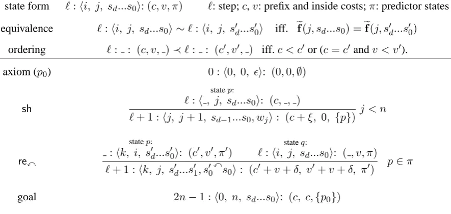
Figure 3: Deductive system for shift-reduce parsing with dynamic programming. The predictor state setπ is an implicit graph-structured stack (Tomita, 1988) while the prefix costcis inspired by Stolcke (1995). The re
ycase is similar, replacings′0xs0 withs′0ys0, and λwithρ = w·fre
y(j, sd...s0). Irrelevant
information in a deduction step is marked as an underscore ( ) which means “can match anything”.
tag of the next wordq1. Since the queue is static
information to the parser (unlike the stack, which changes dynamically), we can usejto replace fea-tures from the queue. So in general we write
ef(j, S) = (j,fd(sd), . . . ,f0(s0))
if the feature window looks at top d+ 1 trees on stack, and wherefi(si)extracts kernel features from treesi(0≤i≤d). For example, for the full
model in Table 1(a) we have
ef(j, S) = (j,f2(s2),f1(s1),f0(s0)), (5)
whered = 2,f2(x) = x.t, andf1(x) = f0(x) = (x.w, x.t, x.lc.t, x.rc.t)(see Table 1(c)).
3.2 Graph-Structured Stack and Deduction
Now that we have the kernel feature functions, it is intuitive that we might only need to remember the relevant bits of information from only the last
(d+ 1)trees on stack instead of the whole stack, because they provide all the relevant information for the features, and thus determine the costs. For shift, this suffices as the stack grows on the right; but for reduce actions the stack shrinks, and in or-der still to maintaind+ 1trees, we have to know something about the history. This is exactly why we needed the full stack for vanilla shift-reduce
parsing in the first place, and why dynamic pro-gramming seems hard here.
To solve this problem we borrow the idea of “graph-structured stack” (GSS) from Tomita (1991). Basically, each statepcarries with it a set π(p) of predictor states, each of which can be combined withpin a reduction step. In a shift step, if statep generates stateq (we say “ppredictsq” in Earley (1970) terms), thenpis added ontoπ(q). When two equivalent shifted states get merged, their predictor states get combined. In a reduction step, stateq tries to combine with every predictor state p ∈ π(q), and the resulting state r inherits the predictor states set from p, i.e.,π(r) = π(p). Interestingly, when two equivalent reduced states get merged, we can prove (by induction) that their predictor states are identical (proof omitted).
Figure 3 shows the new deductive system with dynamic programming and GSS. A new state has the form
ℓ:hi, j, sd...s0i
where [i..j] is the span of the top tree s0, and
sd..s1 are merely “left-contexts”. It can be
com-bined with some predictor statepspanning[k..i]
ℓ′:hk, i, s′d...s′0i
This style resembles CKY and Earley parsers. In fact, the chart in Earley and other agenda-based parsers is indeed a GSS when viewed left-to-right. In these parsers, when a state is popped up from the agenda, it looks for possible sibling states that can combine with it; GSS, however, explicitly maintains these predictor states so that the newly-popped state does not need to look them up.4
3.3 Correctness and Polynomial Complexity
We state the main theoretical result with the proof omitted due to space constraints:
Theorem 1. The deductive system is optimal and
runs in worst-case polynomial time as long as the kernel feature function satisfies two properties:
• bounded:ef(j, S) = (j,fd(sd), . . . ,f0(s0))
for some constant d, and each |ft(x)| also
bounded by a constant for all possible treex.
• monotonic: ft(x) = ft(y) ⇒ ft+1(x) = ft+1(y), for alltand all possible treesx,y.
Intuitively, boundedness means features can only look at a local window and can only extract bounded information on each tree, which is always the case in practice since we can not have infinite models. Monotonicity, on the other hand, says that features drawn from trees farther away from the top should not be more refined than from those closer to the top. This is also natural, since the in-formation most relevant to the current decision is always around the stack top. For example, the ker-nel feature function in Eq. 5 is bounded and mono-tonic, sincef2is less refined thanf1andf0.
These two requirements are related to grammar refinement by annotation (Johnson, 1998), where annotations must be bounded and monotonic: for example, one cannot refine a grammar by only remembering the grandparent but not the parent symbol. The difference here is that the annotations are not vertical ((grand-)parent), but rather hori-zontal (left context). For instance, a context-free rule A → B C would become DA → DB BC
for some D if there exists a rule E → αDAβ. This resembles the reduce step in Fig. 3.
The very high-level idea of the proof is that boundedness is crucial for polynomial-time, while monotonicity is used for the optimal substructure property required by the correctness of DP.
4In this sense, GSS (Tomita, 1988) is really not a new in-vention: an efficient implementation of Earley (1970) should already have it implicitly, similar to what we have in Fig. 3.
3.4 Beam Search based on Prefix Cost
Though the DP algorithm runs in polynomial-time, in practice the complexity is still too high, esp. with a rich feature set like the one in Ta-ble 1. So we apply the same beam search idea from Sec. 2.3, where each step can accommodate only the best b states. To decide the ordering of states in each beam we borrow the concept of
pre-fix cost from Stolcke (1995), originally developed
for weighted Earley parsing. As shown in Fig. 3, the prefix costcis the total cost of the best action sequence from the initial state to the end of statep, i.e., it includes both the inside costv (for Viterbi inside derivation), and the cost of the (best) path leading towards the beginning of statep. We say that a statepwith prefix costcis better than a state p′ with prefix costc′, notatedp ≺ p′ in Fig. 3, if
c < c′. We can also prove (by contradiction) that
optimizing for prefix cost implies optimal inside cost (Nederhof, 2003, Sec. 4).5
As shown in Fig. 3, when a state q with costs
(c, v) is combined with a predictor state p with costs(c′, v′), the resulting staterwill have costs
(c′+v+δ, v′+v+δ),
where the inside cost is intuitively the combined inside costs plus an additional combo costδ from the combination, while the resulting prefix cost c′+v+δ is the sum of the prefix cost of the pre-dictor stateq, the inside cost of the current statep, and the combo cost. Note the prefix cost ofqis ir-relevant. The combo cost δ = ξ′ +λconsists of shift costξ′ofpand reduction costλofq.
The cost in the non-DP shift-reduce algorithm (Fig. 1) is indeed a prefix cost, and the DP algo-rithm subsumes the non-DP one as a special case where no two states are equivalent.
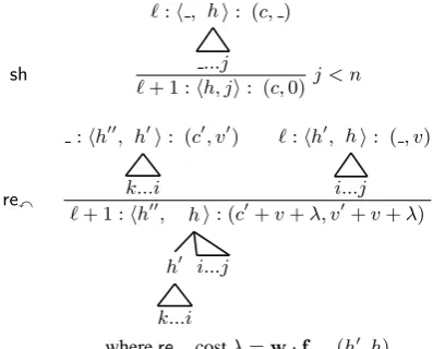
3.5 Example: Edge-Factored Model
As a concrete example, Figure 4 simulates an edge-factored model (Eisner, 1996; McDonald et al., 2005a) using shift-reduce with dynamic pro-gramming, which is similar to bilexical PCFG parsing using CKY (Eisner and Satta, 1999). Here the kernel feature function is
e
f(j, S) = (j, h(s1), h(s0))
sh
ℓ:h, h ...j
i: (c, )
ℓ+ 1 :hh, ji: (c,0)j < n
re
x
:hh′′, h′
k...i
i: (c′, v′) ℓ:hh′, h
i...j
i: (, v)
ℓ+ 1 :hh′′, h
h′
k...i i...j
i: (c′+v+λ, v′+v+λ)
wherere
xcostλ=w·fre
[image:6.595.77.276.62.222.2]x(h ′, h)
Figure 4: Example of shift-reduce with dynamic programming: simulating an edge-factored model. GSS is implicit here, andre
ycase omitted.
whereh(x)returns the head word index of treex, because all features in this model are based on the head and modifier indices in a dependency link. This function is obviously bounded and mono-tonic in our definitions. The theoretical complexity of this algorithm isO(n7
)because in a reduction step we have three span indices and three head in-dices, plus a step index ℓ. By contrast, the na¨ıve CKY algorithm for this model isO(n5
)which can be improved toO(n3
)(Eisner, 1996).6The higher complexity of our algorithm is due to two factors: first, we have to maintain both h and h′ in one state, because the current shift-reduce model can not draw features across different states (unlike CKY); and more importantly, we group states by step ℓin order to achieve incrementality and lin-ear runtime with beam slin-earch that is not (easily) possible with CKY or MST.
4 Experiments
We first reimplemented the reference shift-reduce parser of Huang et al. (2009) in Python (hence-forth “non-DP”), and then extended it to do dy-namic programing (henceforth “DP”). We evalu-ate their performances on the standard Penn Tree-bank (PTB) English dependency parsing task7 us-ing the standard split: secs 02-21 for trainus-ing, 22 for development, and 23 for testing. Both DP and non-DP parsers use the same feature templates in Table 1. For Secs. 4.1-4.2, we use a baseline model trained with non-DP for both DP and non-DP, so that we can do a side-by-side comparison of search
6
OrO(n2)
with MST, but including non-projective trees. 7Using the head rules of Yamada and Matsumoto (2003).
quality; in Sec. 4.3 we will retrain the model with DP and compare it against training with non-DP.
4.1 Speed Comparisons
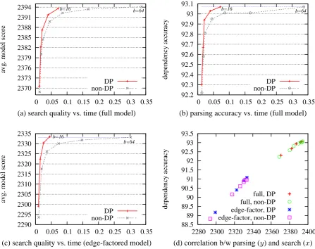
To compare parsing speed between DP and non-DP, we run each parser on the development set, varying the beam widthbfrom 2 to 16 (DP) or 64 (non-DP). Fig. 5a shows the relationship between search quality (as measured by the average model score per sentence, higher the better) and speed (average parsing time per sentence), where DP with a beam width of b=16 achieves the same search quality with non-DP atb=64, while being 5 times faster. Fig. 5b shows a similar comparison for dependency accuracy. We also test with an edge-factored model (Sec. 3.5) using feature tem-plates (1)-(3) in Tab. 1, which is a subset of those in McDonald et al. (2005b). As expected, this dif-ference becomes more pronounced (8 times faster in Fig. 5c), since the less expressive feature set makes more states “equivalent” and mergeable in DP. Fig. 5d shows the (almost linear) correlation between dependency accuracy and search quality, confirming that better search yields better parsing.
4.2 Search Space, Forest, and Oracles
DP achieves better search quality because it ex-pores an exponentially large search space rather than onlybtrees allowed by the beam (see Fig. 6a). As a by-product, DP can output a forest encoding these exponentially many trees, out of which we can draw longer and better (in terms of oracle)k -best lists than those in the beam (see Fig. 6b). The forest itself has an oracle of 98.15 (as ifk→ ∞), computed `a la Huang (2008, Sec. 4.1). These can-didate sets may be used for reranking (Charniak and Johnson, 2005; Huang, 2008).8
4.3 Perceptron Training and Early Updates
Another interesting advantage of DP over non-DP is the faster training with perceptron, even when both parsers use the same beam width. This is due to the use of early updates (see Sec. 2.3), which happen much more often with DP, because a gold-standard statepis often merged with an equivalent (but incorrect) state that has a higher model score, which triggers update immediately. By contrast, in non-DP beam search, states such asp might still
2370 2373 2376 2379 2382 2385 2388 2391 2394
0 0.05 0.1 0.15 0.2 0.25 0.3 0.35
avg. model score
b=16 b=64
DP non-DP
92.2 92.3 92.4 92.5 92.6 92.7 92.8 92.9 93 93.1
0 0.05 0.1 0.15 0.2 0.25 0.3 0.35
dependency accuracy
b=16 b=64
DP non-DP
(a) search quality vs. time (full model) (b) parsing accuracy vs. time (full model)
2290 2295 2300 2305 2310 2315 2320 2325 2330 2335
0 0.05 0.1 0.15 0.2 0.25 0.3 0.35
avg. model score
b=16
b=64
DP non-DP
88.5 89 89.5 90 90.5 91 91.5 92 92.5 93 93.5
2280 2300 2320 2340 2360 2380 2400
dependency accuracy
full, DP full, non-DP edge-factor, DP edge-factor, non-DP
[image:7.595.72.520.85.439.2](c) search quality vs. time (edge-factored model) (d) correlation b/w parsing (y) and search (x)
Figure 5: Speed comparisons between DP and non-DP, with beam sizebranging 2∼16 for DP and 2∼64 for non-DP. Speed is measured by avg. parsing time (secs) per sentence onxaxis. With the same level of search quality or parsing accuracy, DP (atb=16) is∼4.8 times faster than non-DP (atb=64) with the full model in plots (a)-(b), or∼8 times faster with the simplified edge-factored model in plot (c). Plot (d) shows the (roughly linear) correlation between parsing accuracy and search quality (avg. model score).
100 102 104 106 108 1010 1012
0 10 20 30 40 50 60 70
number of trees explored
sentence length DP forest non-DP (16)
93 94 95 96 97 98 99
64 32
16 8 4 1
oracle precision
k
DP forest (98.15) DP k-best in forest non-DP k-best in beam
(a) sizes of search spaces (b) oracle precision on dev
[image:7.595.79.518.549.722.2]90.5 91 91.5 92 92.5 93 93.5
0 4 8 12 16 20 24
accuracy on dev (each round)
hours 17th
18th
[image:8.595.305.525.62.130.2]DP non-DP
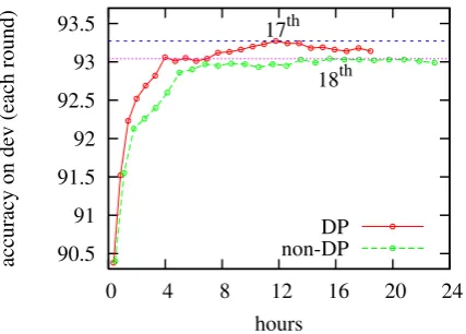
Figure 7: Learning curves (showing precision on dev) of perceptron training for 25 iterations (b=8). DP takes 18 hours, peaking at the 17th iteration (93.27%) with 12 hours, while non-DP takes 23 hours, peaking at the 18th (93.04%) with 16 hours.
survive in the beam throughout, even though it is no longer possible to rank the best in the beam.
The higher frequency of early updates results in faster iterations of perceptron training. Table 2 shows the percentage of early updates and the time per iteration during training. While the number of updates is roughly comparable between DP and non-DP, the rate of early updates is much higher with DP, and the time per iteration is consequently shorter. Figure 7 shows that training with DP is about 1.2 times faster than non-DP, and achieves +0.2% higher accuracy on the dev set (93.27%).
Besides training with gold POS tags, we also trained on noisy tags, since they are closer to the test setting (automatic tags on sec 23). In that case, we tag the dev and test sets using an auto-matic POS tagger (at 97.2% accuracy), and tag the training set using four-way jackknifing sim-ilar to Collins (2000), which contributes another +0.1% improvement in accuracy on the test set. Faster training also enables us to incorporate more features, where we found more lookahead features (q2) results in another +0.3% improvement.
4.4 Final Results on English and Chinese
Table 3 presents the final test results of our DP parser on the Penn English Treebank, compared with other state-of-the-art parsers. Our parser achieves the highest (unlabeled) dependency ac-curacy among dependency parsers trained on the Treebank, and is also much faster than most other parsers even with a pure Python implementation
[image:8.595.74.288.64.217.2]it update early% time update early% time 1 31943 98.9 22 31189 87.7 29 5 20236 98.3 38 19027 70.3 47 17 8683 97.1 48 7434 49.5 60 25 5715 97.2 51 4676 41.2 65
Table 2: Perceptron iterations with DP (left) and non-DP (right). Early updates happen much more often with DP due to equivalent state merging, which leads to faster training (time in minutes).
word L time comp. McDonald 05b 90.2 Ja 0.12 O(n2
)
McDonald 05a 90.9 Ja 0.15 O(n3 )
Koo 08base 92.0 − − O(n4)
Zhang 08single 91.4 C 0.11 O(n)‡
this work 92.1 Py 0.04 O(n)
†Charniak 00 92.5 C 0.49 O(n5)
†Petrov 07 92.4 Ja 0.21 O(n3 )
Zhang 08combo 92.1 C − O(n2 )‡
Koo 08semisup 93.2 − − O(n4 )
Table 3: Final test results on English (PTB). Our parser (in pure Python) has the highest accuracy among dependency parsers trained on the Tree-bank, and is also much faster than major parsers.
†converted from constituency trees. C=C/C++,
Py=Python, Ja=Java. Time is in seconds per sen-tence. Search spaces:‡linear; others exponential.
[image:8.595.308.524.206.343.2]0 0.2 0.4 0.6 0.8 1 1.2 1.4
0 10 20 30 40 50 60 70
parsing time (secs)
sentence length
[image:9.595.77.269.67.213.2]Cha Berk MST DP
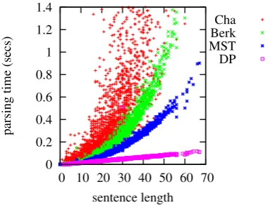
Figure 8: Scatter plot of parsing time against sen-tence length, comparing with Charniak, Berkeley, and theO(n2)MST parsers.
word non-root root compl. Duan 07 83.88 84.36 73.70 32.70 Zhang 08† 84.33 84.69 76.73 32.79
this work 85.20 85.52 78.32 33.72
Table 4: Final test results on Chinese (CTB5).
†The transition parser in Zhang and Clark (2008).
1136), development (secs 886-931 and 1148-1151), and test (secs 816-885 and 1137-1147) sets, assume gold-standard POS-tags for the input, and use the head rules of Zhang and Clark (2008). Ta-ble 4 summarizes the final test results, where our work performs the best in all four types of (unla-beled) accuracies: word, non-root, root, and com-plete match (all excluding punctuations).9,10 5 Related Work
This work was inspired in part by Generalized LR parsing (Tomita, 1991) and the graph-structured stack (GSS). Tomita uses GSS for exhaustive LR parsing, where the GSS is equivalent to a dy-namic programming chart in chart parsing (see Footnote 4). In fact, Tomita’s GLR is an in-stance of techniques for tabular simulation of non-deterministic pushdown automata based on deduc-tive systems (Lang, 1974), which allow for cubic-time exhaustive shift-reduce parsing with context-free grammars (Billot and Lang, 1989).
Our work advances this line of research in two aspects. First, ours is more general than GLR in
9
Duan et al. (2007) and Zhang and Clark (2008) did not report word accuracies, but those can be recovered given non-root and non-root ones, and the number of non-punctuation words. 10Parser combination in Zhang and Clark (2008) achieves a higher word accuracy of 85.77%, but again, it is not directly comparable to our work.
that it is not restricted to LR (a special case of shift-reduce), and thus does not require building an LR table, which is impractical for modern gram-mars with a large number of rules or features. In contrast, we employ the ideas behind GSS more flexibly to merge states based on features values, which can be viewed as constructing an implicit LR table on-fly. Second, unlike previous the-oretical results about cubic-time complexity, we achieved linear-time performance by smart beam search with prefix cost inspired by Stolcke (1995), allowing for state-of-the-art data-driven parsing.
To the best of our knowledge, our work is the first linear-time incremental parser that performs dynamic programming. The parser of Roark and Hollingshead (2009) is also almost linear time, but they achieved this by discarding parts of the CKY chart, and thus do achieve incrementality.
6 Conclusion
We have presented a dynamic programming al-gorithm for shift-reduce parsing, which runs in linear-time in practice with beam search. This framework is general and applicable to a large-class of shift-reduce parsers, as long as the feature functions satisfy boundedness and monotonicity. Empirical results on a state-the-art dependency parser confirm the advantage of DP in many as-pects: faster speed, larger search space, higher ora-cles, and better and faster learning. Our final parser outperforms all previously reported dependency parsers trained on the Penn Treebanks for both English and Chinese, and is much faster in speed (even with a Python implementation). For future work we plan to extend it to constituency parsing.
Acknowledgments
References
Alfred V. Aho and Jeffrey D. Ullman. 1972. The
Theory of Parsing, Translation, and Compiling, vol-ume I: Parsing of Series in Automatic Computation. Prentice Hall, Englewood Cliffs, New Jersey.
S. Billot and B. Lang. 1989. The structure of shared forests in ambiguous parsing. In Proceedings of the 27th ACL, pages 143–151.
Eugene Charniak and Mark Johnson. 2005.
Coarse-to-fine-grained n-best parsing and discriminative
reranking. In Proceedings of the 43rd ACL, Ann Ar-bor, MI.
Eugene Charniak. 2000. A
maximum-entropy-inspired parser. In Proceedings of NAACL.
Michael Collins and Brian Roark. 2004. Incremental parsing with the perceptron algorithm. In Proceed-ings of ACL.
Michael Collins. 2000. Discriminative reranking for natural language parsing. In Proceedings of ICML, pages 175–182.
Michael Collins. 2002. Discriminative training meth-ods for hidden markov models: Theory and experi-ments with perceptron algorithms. In Proceedings of EMNLP.
Xiangyu Duan, Jun Zhao, and Bo Xu. 2007. Proba-bilistic models for action-based chinese dependency parsing. In Proceedings of ECML/PKDD.
Jay Earley. 1970. An efficient context-free parsing al-gorithm. Communications of the ACM, 13(2):94– 102.
Jason Eisner and Giorgio Satta. 1999. Efficient pars-ing for bilexical context-free grammars and head-automaton grammars. In Proceedings of ACL.
Jason Eisner. 1996. Three new probabilistic models
for dependency parsing: An exploration. In
Pro-ceedings of COLING.
Lyn Frazier and Keith Rayner. 1982. Making and cor-recting errors during sentence comprehension: Eye movements in the analysis of structurally ambigu-ous sentences. Cognitive Psychology, 14(2):178 – 210.
Liang Huang and David Chiang. 2005. Betterk-best
Parsing. In Proceedings of the Ninth International Workshop on Parsing Technologies (IWPT-2005).
Liang Huang, Wenbin Jiang, and Qun Liu. 2009.
Bilingually-constrained (monolingual) shift-reduce parsing. In Proceedings of EMNLP.
Liang Huang. 2008. Forest reranking: Discriminative parsing with non-local features. In Proceedings of the ACL: HLT, Columbus, OH, June.
Mark Johnson. 1998. PCFG models of
linguis-tic tree representations. Computational Linguislinguis-tics, 24:613–632.
Terry Koo, Xavier Carreras, and Michael Collins. 2008. Simple semi-supervised dependency parsing. In Proceedings of ACL.
B. Lang. 1974. Deterministic techniques for efficient non-deterministic parsers. In Automata, Languages and Programming, 2nd Colloquium, volume 14 of Lecture Notes in Computer Science, pages 255–269, Saarbr¨ucken. Springer-Verlag.
Lillian Lee. 2002. Fast context-free grammar parsing requires fast Boolean matrix multiplication. Journal of the ACM, 49(1):1–15.
Ryan McDonald, Koby Crammer, and Fernando Pereira. 2005a. Online large-margin training of de-pendency parsers. In Proceedings of the 43rd ACL.
Ryan McDonald, Fernando Pereira, Kiril Ribarov, and Jan Hajiˇc. 2005b. Non-projective dependency pars-ing uspars-ing spannpars-ing tree algorithms. In Proc. of HLT-EMNLP.
Mark-Jan Nederhof. 2003. Weighted deductive pars-ing and Knuth’s algorithm. Computational Lpars-inguis- Linguis-tics, pages 135–143.
Joakim Nivre. 2004. Incrementality in deterministic dependency parsing. In Incremental Parsing: Bring-ing EngineerBring-ing and Cognition Together. Workshop at ACL-2004, Barcelona.
Slav Petrov and Dan Klein. 2007. Improved inference for unlexicalized parsing. In Proceedings of HLT-NAACL.
Brian Roark and Kristy Hollingshead. 2009. Linear complexity context-free parsing pipelines via chart constraints. In Proceedings of HLT-NAACL.
Andreas Stolcke. 1995. An efficient
probabilis-tic context-free parsing algorithm that computes
prefix probabilities. Computational Linguistics,
21(2):165–201.
Masaru Tomita. 1988. Graph-structured stack and nat-ural language parsing. In Proceedings of the 26th annual meeting on Association for Computational Linguistics, pages 249–257, Morristown, NJ, USA. Association for Computational Linguistics.
Masaru Tomita, editor. 1991. Generalized LR Parsing. Kluwer Academic Publishers.
H. Yamada and Y. Matsumoto. 2003. Statistical de-pendency analysis with support vector machines. In Proceedings of IWPT.
Yue Zhang and Stephen Clark. 2008. A tale of