Munich Personal RePEc Archive
High dimensional Global Minimum
Variance Portfolio
Li, Hua and Bai, Zhi Dong and Wong, Wing Keung
Department of Science, Chang Chun University„ School of
Mathematics and Statistics, Northeast Normal University,
Department of Economic, Hong Kong Baptist University
26 August 2015
Online at
https://mpra.ub.uni-muenchen.de/66284/
High dimensional Global Minimum Variance Portfolio
Li Hua
1, Bai Zhidong
2, and Wong-Wing Keung
31Department of Science, Chang Chun University, [email protected]
2School of Mathematics and Statistics, Northeast Normal University, [email protected] 3Department of Economic, Hong Kong Baptist University, [email protected]
Abstract: This paper proposes the spectral corrected methodology to estimate the Global Minimum Variance Portfolio (GMVP) for the high dimensional data. In this paper, we analysis the limiting properties of the spectral corrected GMVP estimator as the dimension and the number of the sample set increase to infinity proportionally. In addition, we compare the spectral corrected estimation with the linear shrinkage and nonlinear shrinkage estimations and obtain that the performance of the spectral corrected methodology is best in the simulation study.
Keyword: Global Minimum Variance Portfolio, Spectral Corrected Covariance, Sample Covariance
1 Introduction
Since Markowitz mean-variance (MV) portfolio has been invented in 1952, it has become a cor-nerstone of modern finance. This theory incorpo-rates the investors’ preference and their expecta-tion of returns and risks. By this theory, investors could construct the optimal portfolio by minimiz-ing the portfolio variance for a given level of the expected return or maximizing the portfolio return for a given level of the portfolio risk. In MV portfo-lio theory the global minimum variance portfoportfo-lio (GMVP) is a remarkable and mostly useful portfo-lio. This portfolio has the smallest variance over all portfolios and do not depend on the expected return. In fact, much empirical work reports un-derperformance of market capitalisation-weighted portfolios relatives to the GMV portfolio (Clarke et al. [2006], Baker et al. [2011] and so on).
Suppose there are p assets and ri be the
ran-dom return of the ith one (i = 1, ...,p). Denote
w= (ω1, ..., ωp)′ as an asset allocation. Then the
theoretical GMVP is the unique solution of the fol-lowing quadratic program:
minimize w′
Σpw subject to w
′
1= 1. (1)
Here1is a vector of which the elements are1s and Σpstands for the covariance matrix of the random
return vectorr= (r1, ...,rp)′. Then the theoretical
GMVP
wo=
Σ−1 p 1 1′Σ−1
p 1
, (2)
the expected GMVP return Ro = µ′Σp−11/1′Σ−p11
and the GMVP riskσ2o = 1/1
′Σ−1 p 1.
There are a great deal of papers to estimate GMVP (see Kempf and Memmel [2003], Bodnar and Schmid [2008], Bodnar and Schmid [2007], Frahm and Memmel [2010], Clarke et al. [2011], Bodnar and Gupta [2012], Wied et al. [2013], Green et al. [2013] and so on). GMVP has nice theoretical properties in many ways, but it is in-evitable to estimate the population covariance matrix of the random returns in practice. The classical estimator is usually constructed by plug-ging the sample covariance matrix into GMVP ex-pression (2) instead of the unknown parameter Σp. When the number of observations n is large
enough compared with the number of assetsp, the
sample covariance matrix is not bad choice (see Okhrin and Schmid [2006], Memmel and Kempf, Bodnar and Schmid [2009] and so on), but it tends to be far from the population covariance matrix (Bai et al. [2004]) when the number of assets p
can not be ignored with respect to the sample size
nand thus it is not a appropriate estimator ofΣ. Whenpis large compared with the sample size n, how to estimate a covariance matrix and/or
or even more years (Bickel and Levina [2008], Cai and Zhou [2012], Rohde et al. [2011], Khare et al. [2011], Rajaratnam et al. [2008], Fan et al. [2008],Ledoit and Wolf [2004a] , Ledoit and Wolf [2004b], Golosnoy and Okhrin [2007], Frahm and Memmel [2010] and so on ).
In this paper, we estimate GMVP for the high dimensional data by the spectral corrected Methodology. Here we propose the spectral cor-rected covariance as the population covariance es-timator and plug it into (2). In this paper, we com-pare the spectral corrected estimation with the classic estimation, the linear shrinkage estimation and the nonlinear shrinkage estimation and find the performance of the spectral corrected estima-tion is best in the simulaestima-tion study.
In Section 2, we will introduce the spectral cor-rected estimation for GMVP. In Sections 3 and 4, the Linear shrinkage estimation and the nonlinear shrinkage estimation are provided. We provide the simulation study in Section 5 and the conclu-sion in Section 6.
2 Spectral corrected
estima-tion
In this part we develop the spectral corrected GMVP by plugging the spectral-corrected covari-ance as the estimation ofΣp into (2). The
spec-tral corrected covariance is constructed by correct-ing the spectrum of the sample covariance ma-trix. Suppose that x1,x2, ...,xn are identified
in-dependent distributed (i.i.d.) pdimensional
ran-dom return vectors with the meanµ and the
co-variance matrixΣp. Write the spectral
decomposi-tion of the sample covarianceSn =∑ni=1xix′−x x
′
can as TnΛnT′n where Λn = diag{λn,1, λn,2, ..., λn,p}
(λn,1 ≥ λn,2 ≥... ≥λn,p) andTn is the matrix with
the corresponding eigenvectors.
For any symmetry matrixAwith the dimension
p, define the empirical spectral distribution (SD)
as following
FA(x) = 1
p p
∑
i=1
1[λi,∞)(x), x∈R (3)
in which λ1 ≥ λ2 ≥ ... ≥ λp are the
eigenval-ues of Aand 1[λi,∞)(x)equals to 1 forλi ≤ xand
0otherwise. Then according to the large dimen-sional random matrix theory, under some
reason-able conditions, FSn weakly converges to a
de-terministic distribution F as p and n increase to
infinity proportionally, which is called limiting spectral distribution (LSD) (Marčenko and Pastur [1967], Silverstein [1995] and Silverstein and Bai [1995]). Denote the stieltjes transform of F as m(z) = ∫(x−z)−1dF(x)(z∈ Candℑz,0). Then
m(z)is the unique solution of
z(m) = 1
m(z)+y
∫ t
1 +tmdH(t) (4)
on the upper half complex plane in which H is
the limiting spectral distribution of the population covariance matrix Σp and m = −(1−y)/z+ym
(z ∈ C+). (4) provides a chance to recover the
spectral information of the population covariance Σp. Mestre [2008] and Li and Yao [2013]
pro-vide the spectral estimation based on the contour integration under eigenvalue splitting condition and no splitting condition, respectively. Karoui [2008], Rao et al. [2008] , Chen et al. [2011] and so on introduce more methods to estimate the spectral construction of the populationΣp.
In this paper, we do not focus on the estima-tion ofFΣp and suppose the spectral construction
ofΣp is known or estimated well. We correct the
spectrum of the sample covariance and obtain the spectral corrected varianceeSn=Tn∆pT′n in which
∆p =diag{τ1, ..., τp}andτ1 ≥...≥τp are the
spec-tral elements of Σp. Compared with the quartic
form of the sample covariance matrix inverse, that of the spectral corrected covariance one performs more stably in the simulation study. We explain more details in the Theorem 2.1 and 2.2 under some reasonable assumptions:
Assumption 2.1. Yn = (y1,· · ·,yn) = (yi,j)p,n in
whichyi,j (i = 1,· · ·,p,j = 1,· · · ,n)are i.i.d.
ran-dom variables withEyi j= 0,E|yi j|2= 1,E|yi j|4<∞,
andxk= Σ
1/2
p ykfor eachnand fork= 1,2,· · ·,n; Assumption 2.2. ap,bp ∈Cp ={x∈ Cp}are
uni-formly bounded vectors.
Assumption 2.3. Σp = Up∆pU∗p is nonrandom
symmetry and nonnegative definite with its spectral
norm bounded in pwhere
∆p=diag(τ1I1, τ2I2, ..., τLIL) (5)
τ1> τ2>· · ·> τL,Up= (Up,1,Up,2,· · ·,Up,L)andIi
Theorem 2.1. Under Assumptions from 2.1 to 2.3, asp,n→ ∞,p/n→y,(0<y<1), we have
a′pS−1 n bp ap′Σ−p1bp
−→ 1
(1−y) a.s. (6)
According to Theorem 2.1, a′pS−1
n bp is
asymp-totically(1−y)−1time ofa′
pΣ
−1
p bpand wheny→1, a′pS−1
n bp is close to infinity. This is because the
minimum eigenvalue of the sample covariance is very close to zero asy → 1 and thus its inverse goes to infinity which mainly decides the value of
a′pS−1
n bp. Then it is a natural idea of correcting
eigenvalues ofSn to be the spectral corrected
co-varianceeSn. The following theorem explains the
limiting behavior about the quartic forma′
peS
−1 n bp
under general conditions.
Theorem 2.2. Suppose the limiting spectral distribution of Sn is spectral separated and a′pU
p,iUTp,ibp = fi(i= 1,2,· · ·,L). Under
Assump-tions 2.1 to 2.3, we have
a′
peS
−1 n bp−→
L
∑
k=1
fkdk a.s. (7)
asp,n→ ∞and p/n→y. Heredk=∑Lj=1 (uj−τj)
τj(uj−τk)
andujis the solution of1+y
∫ t
u−tdH(t) = 0for any j= 1,· · ·,Lwithτ1>u1> τ2>· · ·> τL>uL>0.
Note: in (7), it is difficult to explain the rela-tionship between the limiting behaves ofa′pS−1
n bp
anda′eS−1
n bp theoretically. In this paper, we
pro-vide some Monte-Carlo experiments to describe the performance ofa′
peS−n1bpand the conclusion of
Theorem 2.1 and 2.2.
For the population covarianceΣp, select series
{
ap
}
and{bp
}
such thata′
pΣ
−1
p bp is a constant for
any dimensionp. Generate the sample setX1, ...Xn
from the population with a non zero meanµand
the covariance matrix Σp and compute a′pS−n1bp
anda′
peS
−1
n bp. Here we use τ = [τ1, τ2, ..., τk]and
w = [w1,w2, ...,wp] (wi = pi/p, i = 1,2, ...,p) to
denote the different eigenvalues of Σp and the
corresponding weights on the wholepdimension.
Repeat this process for N times and report their means and the standard deviations in Table 1.
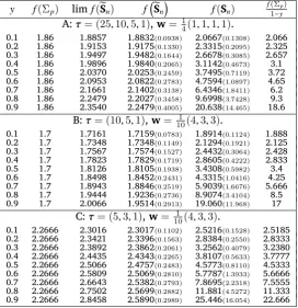
From Table 1, we can find some better perfor-mances of the spectral corrected covariance than that of the sample covariance in the estimation of the quartic form a′
pΣ
−1
p bp. First, the estimate of a′
peS
−1
n bpis more accurate than that ofa′pS−n1bp. In
Table 1, for a given a′
pΣ−P1bp, the average error
ofa′
peS
−1
n bp is very small asy= 0.1 and increases
slowly with the increasing ofyfrom0.1to0.9but still is bounded by0.5in all three Panels. For the sample covariance, the average error of a′pS−1
n bp
is smallest when y = 0.1 and still is about0.2 in Panel A, B and C. It increases with increasing ofy
from0.1to0.9 rapidly. Wheny= 0.9,a′pS−1 n bp is
asymptotically ten times ofa′
pΣ−p1bp. In addition,
the estimate of a′pS−1
n bp is much unstabler
com-pared with that ofa′
peS
−1
n bpaccording to their
dard deviation reports. Though both of the stan-dard deviations associated witheSnandSnincrease
as the increasing ofy, the largest one ofa′peS−n1bpis
still not more than0.4while that ofa′pS
nbpalready
reaches16.
From above analysis and the simulation study, it is natural to plugeSninto (2) and have the
spec-tral corrected global minimum variance portfolio (SCGMVP) as follows:
e
wsc=
eS−1 n 1 1′eS−1
n 1
. (8)
Then the expected return of SCGMVPRsc=µ′wesc
and the corresponding riskσ2sc=we′scΣpwesc. In the
structure ofwesc, the eigenvector matrixTn is the
main random part and determines the final perfor-mance of SCGMV.
Corollary 2.1. Under the conditions of Theorem 2.2,
Rsc Ro
→
∑L
i,j=1 fr,if1,jdiτj
∑L
i,j=1 fr,if1,jdjτi
a.s.
asp,n→ ∞and p/n→y. Heredi(i= 1, ...,L) are
defined in Theorem 2.2.
The proof of Corollary 2.1 can be deduced by Theorem 2.1 and 2.2 directly.
By the spectral corrected methodology, we can not obtain a portfolio estimator with a consistent expected return as Ro, but SCGMVP has higher
3 Linear shrinkage Estimation
Ledoit and Wolf [2004b] propose a well condi-tioned estimator for large dimensional covariance matrices. In this paper, they focus on the optimal linear combinationΣ∗=ρ
1I+ρ2Snof the identity
matrix I and the sample covariance matrix who minimizes the expected quadratic lossE∥Σ∗−Σ∥2
for allρ1, ρ2∈R. That is
min
ρ1,ρ2E∥Σ
∗
−Σ∥2 s.t. Σ∗=ρ1I+ρ2Sn. (9)
Here ∥ · ∥ is the Frobenius norm: ∥M∥ =
√
Tr(MM′)/rfor anyr×mmatrixM. By the
com-putation, the solution of the optimization problem is
Σ∗=β
2
δ2µI+
α2
δ2Sn (10)
Hereµ=tr(Σ)/p,α2=∥Σ−µI∥2,β2=E∥S n−Σ∥2
andδ2=E∥Sn−µI∥2. By the large dimensional
ran-dom theory, the consistent estimations for these parameters is ˆµ = tr(Sn)/p, δˆ2 = ∥Sn − ˆµI∥2,
ˆ
β2 = min(b2n,ˆδ2n) and αˆn2 = ˆδ2n −βˆ2n where b2n =
1 n2
∑n
k=1∥y·ky′·k−Sn∥ 2andy
·kis thek-th column of
the data matrixYn. Then the corresponding linear
shrinkage estimator is given as
Σn=
ˆ
β2
ˆ
δ2ˆµI+
ˆ
α2
ˆ
δ2Sn.
4 Nonlinear shrinkage
Estima-tion
Nonlinear shrinkage estimation of the covariance matrix was introduced by Ledoit et al. [2012]. Now I will introduce this methodology shortly. Suppose bΣ ≡ bΣ(Yn) be an estimator of Σ under
the data matrixYn. Then for any arbitrary
orthog-onal matrixA, ifΣ(b AYn) =AbΣ(Yn)A, the
estima-tionbΣis said to be rotation-equivariant. With the rotation equivariant property, the estimator ofΣ can be written as the formVnDnV′n whereDn is a
diagonal matrix with elementsd1, ...,dp andVn is
the sample eigenvectors matrix of the data set. In the rotation-equivariant estimator set, Ledoit et al. [2012] consider the optimal estimator under the following loss function
VnDnV′n−Σ (11)
where∥ · ∥is the Frobenius norm defined as∥M∥=
√
Tr(MM′)/r for any r×m matrix M. Minimize
the loss function (11) and get the solution is
D∗
n ≡ Diag(d
∗
1, ...,d
∗
p) where d
∗
i = v
′
iΣvi and vi is i-th column of V for i = 1, ...,p. Then the
opti-mal rotation-equivariant estimator of Σ is S∗
n = VnD∗nV′n.
In fact, the structures of the optimal rotation-equivariant estimator S∗
n = VnD∗nV′n and the
spectral-corrected estimator eSn = Tn∆pT′n are
same. They all keep the eigenvector matrix of sample covariance and change it’s spectral ele-ments and S∗
n has smaller loss than eSn. But the
problem is d∗i (i = 1, ...,p) are unknown even as
the spectral element of Σp is given. It not only
increases the difficulty of estimations but also re-duces the accuracy.
For the estimation ofd∗i (i= 1, ...,p), Ledoit and
Péché [2011] show that they can be approximated by
dori ≡ λi
1−c−cλimˇF(λi)
2. (12)
Hereλiis theith eigenvectvalue of sample
covari-ance,mˇF(λi) = 1cλ−c
i −
1
czλi andzλi is the solution of the following equation
z−cz
∫ +∞ −∞
τ
τ−zdH(τ) =λi for i= 1, ...p and z∈C
+.
According to (12), the oracle estimator is given as
Sor
n =VnDornV
′
n where D or
n ≡Diag(d or
1, ...,d
or p).
By the same way, among the class of rotation-equivant estimators, the optimal estimator of Σ−1
p is given by P
∗
n ≡ VnA∗nV′n where A
∗
n ≡
Diag(a∗1, ...,a∗p). Here a∗i ≡v
′
iΣ
−1v
i and can be
ap-proximated byaor i ≡λ
−1
i (1−c−2cλiRe[ ˇmF(λi)])for
i = 1, ...,p. Then the corresponding oracle
esti-mator ofΣ−1 is given asPor
n ≡ VnAorn Vn in which Aor
n =Diag(aor1, ...,aorp).
5 Simulation study
In this part, we compare the behaviors of four esti-mators ofΣp—the spectral-corrected estimatoreSn,
the sample covarianceSn, the linear shrinkage
es-timatorΣnand the nonlinear shrinkage estimators Sor
n andPorn in GMV model. In particular, note that Por
n is the estimator ofΣ
−1and not equal to(Sor n)
Plug the estimators ofΣporΣ−p1intoRoandσ2oand
compare their behaviors in the portfolio expected return and risk.
Suppose there are p assets with a random
return vector r = (r1,r2, ...,rp)′ with nonzero
mean µ = (µ1,· · ·, µp)′ and the covariance
ma-trixΣp. Here we use τ = [τ1, τ2, ..., τk] andw =
[w1,w2, ...,wp](wi = pi/p) to denote the different
eigenvalues ofΣp and the corresponding weights
on the whole pdimension. The simulation is
de-signed in the following steps:
(i) Generateni.i.d. pdimensional sample
vec-torsr1,r2, ...,rn with the meanµand the
co-variance matrixΣp.
(ii) Compute the covariance matrix estimators— the sample covariance Sn, the
spectral-corrected sample covariance eSn, the
lin-ear shrinkage covariance Σn, the nonlinear
shrinkage covariance Sor
n and the nonlinear
shrinkage inverse covariancePor n.
(iii) Plug the covariance estimators into
[
wGMV =
b
Σ−1 p 1 1′bΣ−1
p 1
, Rw[GMV =
µ′bΣ−p11 1′bΣ−1
p 1
in whichbΣp = Sn,eSn,Σn andSorn. Plug the
inverse estimationPor n into
[
wGMV∗= P or n1 1′Por
n1
, Rw[GMV∗=
µ′Porn1 1′Por
n1
.
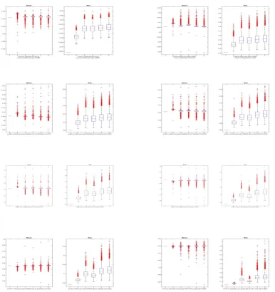
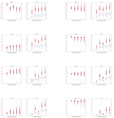
(iv) Repeat steps from (i) to (ii) for N times. Figures 1 and 2 report the expected returns and risks of the GMV portfolio estimates associated with different covariance estimators—the spectral corrected covariance, the sample covariance, the linear shrinkage covariance, the nonlinear shrink-age covariance. In these two figures, we pro-vide 8 pairs of the expected return and risk box plots for two population covariance structures as
y= 0.1,0.2, ...,0.8, respectively. The numbers from
1 to 5 on the x-axes record the expected return and risk of the theoretical GMVP and that of the GMVP estimator associated with the covariance estimators—eSn, Sn, Σn, Sorn andPorn. In these two
figures, the repeating time is 10000 and thus the computation scientific precision is asymptotically down to the second decimal point.
For the expected returns of the GMVP esti-mates, the performance of SCGMVP is not signif-icantly better than the others. The medias of the expected returns of the every estimation almost are located betweenRo±0.01and the interquartile
ranges are smaller than 0.005which means these portfolio estimations perform well without signif-icant differences in the expected return.
For the risks of the GMVP estimates, the perfor-mance of the spectral corrected GMV portfolio is not significant different from the other asy= 0.1 and is significantly better than the others. For all
ys from0.2to 0.8, the media and the correspond-ing interquartile range of the risks associated with the spectral corrected portfolio is smallest com-pared with that of the other estimations. The me-dias of the expected returns of SCGMVP are larger than the theoretical risk of GMVP at least0.02and smaller than the others at least 0.01. According to the interquartile ranges of the risks associated with the GMVP estimators, SCGMVP’s risks are stablest since the difference between the range of SCGMVP’s risks and the others is at least0.02 as
y≥0.2. Thus, from Figures 1 and 2, it is reason-able to use the spectral corrected methodology to estimate the global minimum variance portfolio.
6 Conclusion
In this paper, we introduce the spectral corrected methodology to correct the eigenvalues of the sample covariance matrix and construct the spec-tral corrected global minimum variance portfolio. This methodology overcomes the serious distur-bance deduced by the departure of the spectrum of the sample covariance from that of the popu-lation covariance matrix in the estimation of the global minimum variance portfolio. In addition, compared with the linear shrinkage and nonlin-ear shrinkage estimations, SCGMVP has more ex-pected return and Lower average risk. Therefore, we have enough reason to consider the spectral corrected methodology to construct GMVP estima-tor.
References
sam-ple covariance matrices. The Annals of Probabil-ity, 32(1A):553–605, 2004.
Malcolm P Baker, Brendan Bradley, and Jeffrey Wurgler. Benchmarks as limits to arbitrage: Un-derstanding the low-volatility anomaly. Finan-cial Analysts Journal, 67(1), 2011.
Peter J Bickel and Elizaveta Levina. Regularized estimation of large covariance matrices.The An-nals of Statistics, pages 199–227, 2008.
Taras Bodnar and Arjun K Gupta. Robustness of the inference procedures for the global min-imum variance portfolio weights in a skew-normal model†.The European Journal of Finance, (ahead-of-print):1–19, 2012.
Taras Bodnar and Wolfgang Schmid. The dis-tribution of the sample variance of the global minimum variance portfolio in elliptical mod-els. Statistics, 41(1):65–75, 2007.
Taras Bodnar and Wolfgang Schmid. A test for the weights of the global minimum variance portfo-lio in an elliptical model. Metrika, 67(2):127– 143, 2008.
Taras Bodnar and Wolfgang Schmid. Economet-rical analysis of the sample efficient frontier.
The European journal of finance, 15(3):317–335,
2009.
T Tony Cai and Harrison H Zhou. Minimax estima-tion of large covariance matrices under l1 norm.
Statist. Sinica, 22:1319–1378, 2012.
Jiaqi Chen, Bernard Delyon, and J-F Yao. On a model selection problem from high-dimensional sample covariance matrices. Journal of
Multi-variate Analysis, 102(10):1388–1398, 2011.
Roger Clarke, Harindra De Silva, and Steven Thor-ley. Minimum-variance portfolio composition.
Journal of Portfolio Management, 37(2):31, 2011.
Roger G Clarke, Harindra De Silva, and Steven Thorley. Minimum-variance portfolios in the us equity market. The journal of portfolio manage-ment, 33(1):10–24, 2006.
Jianqing Fan, Yingying Fan, and Jinchi Lv. High dimensional covariance matrix estimation using a factor model. Journal of Econometrics, 147(1): 186–197, 2008.
Gabriel Frahm and Christoph Memmel. Dominat-ing estimators for minimum-variance portfolios.
Journal of Econometrics, 159(2):289–302, 2010.
Vasyl Golosnoy and Yarema Okhrin. Multivariate shrinkage for optimal portfolio weights.The
Eu-ropean Journal of Finance, 13(5):441–458, 2007.
Jeremiah Green, John RM Hand, and X Frank Zhang. The supraview of return predictive sig-nals. Review of Accounting Studies, 18(3):692– 730, 2013.
Noureddine El Karoui. Spectrum estimation for large dimensional covariance matrices using random matrix theory. The Annals of Statistics, pages 2757–2790, 2008.
Alexander Kempf and Christoph Memmel. On the estimation of the global minimum variance portfolio. Available at SSRN 385760, 2003. Kshitij Khare, Bala Rajaratnam, et al. Wishart
dis-tributions for decomposable covariance graph models. The Annals of Statistics, 39(1):514–555, 2011.
Olivier Ledoit and Sandrine Péché. Eigenvectors of some large sample covariance matrix ensem-bles. Probability Theory and Related Fields, 151 (1-2):233–264, 2011.
Olivier Ledoit and Michael Wolf. Honey, i shrunk the sample covariance matrix. The Journal of
Portfolio Management, 30(4):110–119, 2004a.
Olivier Ledoit and Michael Wolf. A well-conditioned estimator for large-dimensional co-variance matrices.Journal of multivariate analy-sis, 88(2):365–411, 2004b.
Olivier Ledoit, Michael Wolf, et al. Nonlinear shrinkage estimation of large-dimensional co-variance matrices. The Annals of Statistics, 40 (2):1024–1060, 2012.
Weiming Li and Jianfeng Yao. A local mo-ment estimator of the spectrum of a large di-mensional covariance matrix. arXiv preprint
arXiv:1302.0356, 2013.
Table 1: Comparison ofa′
pΣ
−1
p bp, limapeSn−1bp,a′peS
−1
n bp,a′pS−n1bpand a
′ pΣ−1bp
1−y . y f(Σp) limf(eSn) f
( eSn
)
f(Sn)
f(Σp)
1−y
A:τ= (25,10,5,1),w=14(1,1,1,1).
0.1 1.86 1.8857 1.8832(0.0938) 2.0667(0.1308) 2.066
0.2 1.86 1.9153 1.9175(0.1330) 2.3315(0.2095) 2.325
0.3 1.86 1.9497 1.9482(0.1644) 2.6678(0.3085) 2.657
0.4 1.86 1.9896 1.9840(0.2065) 3.1142(0.4673) 3.1
0.5 1.86 2.0370 2.0253(0.2459) 3.7495(0.7119) 3.72
0.6 1.86 2.0953 2.0822(0.2783) 4.7594(1.0897) 4.65
0.7 1.86 2.1661 2.1402(0.3138) 6.4346(1.8411) 6.2
0.8 1.86 2.2479 2.2027(0.3458) 9.6998(3.7428) 9.3
0.9 1.86 2.3540 2.2479(0.4005) 20.638(14.465) 18.6
B:τ= (10,5,1),w=101(4,3,3).
0.1 1.7 1.7161 1.7159(0.0783) 1.8914(0.1124) 1.888
0.2 1.7 1.7348 1.7348(0.1149) 2.1294(0.1921) 2.125
0.3 1.7 1.7567 1.7574(0.1527) 2.4432(0.3064) 2.428
0.4 1.7 1.7823 1.7829(0.1719) 2.8605(0.4222) 2.833
0.5 1.7 1.8126 1.8105(0.1938) 3.4308(0.5982) 3.4
0.6 1.7 1.8498 1.8452(0.2431) 4.3315(1.0416) 4.25
0.7 1.7 1.8943 1.8846(0.2519) 5.9039(1.6676) 5.666
0.8 1.7 1.9444 1.9236(0.2736) 8.9074(3.4104) 8.5
0.9 1.7 2.0066 1.9514(0.2913) 19.060(11.968) 17
C:τ= (5,3,1),w= 101(4,3,3).
0.1 2.2666 2.3016 2.3017(0.1102) 2.5216(0.1528) 2.5185
0.2 2.2666 2.3421 2.3396(0.1563) 2.8384(0.2550) 2.8333
0.3 2.2666 2.3892 2.3862(0.2061) 3.2562(0.4079) 3.2380
0.4 2.2666 2.4435 2.4343(0.2265) 3.8107(0.5633) 3.7777
0.5 2.2666 2.5066 2.4757(0.2483) 4.5773(0.8110) 4.5333
0.6 2.2666 2.5809 2.5069(0.2810) 5.7787(1.3933) 5.6666
0.7 2.2666 2.6643 2.5382(0.2793) 7.8695(2.2318) 7.5555
0.8 2.2666 2.7502 2.5699(0.2882) 11.881(4.5272) 11.333
0.9 2.2666 2.8458 2.5890(0.2989) 25.446(16.054) 22.666
Note: here f(A) =a′pA−1b
p,n= 100,y=p/nandN= 10000
Christoph Memmel and Alexander Kempf. Esti-mating the global minimum variance portfolio.
Available at SSRN 940367.
Xavier Mestre. Improved estimation of eigenval-ues and eigenvectors of covariance matrices us-ing their sample estimates. Information Theory,
IEEE Transactions on, 54(11):5113–5129, 2008.
Yarema Okhrin and Wolfgang Schmid. Distribu-tional properties of portfolio weights. Journal
of econometrics, 134(1):235–256, 2006.
Bala Rajaratnam, Hélene Massam, Carlos M Car-valho, et al. Flexible covariance estimation in graphical gaussian models. The Annals of Statis-tics, 36(6):2818–2849, 2008.
N Raj Rao, James A Mingo, Roland Speicher, and Alan Edelman. Statistical eigen-inference from
large wishart matrices. The Annals of Statistics, pages 2850–2885, 2008.
Angelika Rohde, Alexandre B Tsybakov, et al. Esti-mation of high-dimensional low-rank matrices.
The Annals of Statistics, 39(2):887–930, 2011.
Jack W Silverstein. Strong convergence of the em-pirical distribution of eigenvalues of large di-mensional random matrices. Journal of
Multi-variate Analysis, 55(2):331–339, 1995.
Jack W Silverstein and ZD Bai. On the empiri-cal distribution of eigenvalues of a class of large dimensional random matrices. Journal of
Multi-variate analysis, 54(2):175–192, 1995.
Figure 1: Comparetion of the GMV portfolio estimators associated with the spectral-corrected covari-ance, sample covaricovari-ance, linear shrinkage covariance and non-linear shrinkage covariance.
Note: we provide 8 pairs of the expected return and risk box plots fory= 0.1,0.2, ...,0.8. Here the different eigenvalue and
the corresponding weight vectors are(1,5,10)and(0.3,0.4,0.3), respectively. We use the number in the x-axes to denote the
population result and the different estimations in which 1 is the population result and the numbers from 2 to 6 represent the estimations associated witheSn,S,Σn,Sor
Figure 2: Comparetion of the GMV portfolio estimators associated with the spectral-corrected covari-ance, sample covaricovari-ance, linear shrinkage covariance and non-linear shrinkage covariance.
Note: we provide 8 pairs of the expected return and risk box plots fory= 0.1,0.2, ...,0.8. Here the different eigenvalue and
the corresponding weight vectors are(1,3,5)and(0.3,0.4,0.3), respectively. We use the number in the x-axes to denote the
population result and the different estimations in which 1 is the population result and the numbers from 2 to 6 represent the estimations associated witheSn,S,Σn,Sor