Perplexity on Reduced Corpora
Hayato Kobayashi∗ Yahoo Japan Corporation
9-7-1 Akasaka, Minato-ku, Tokyo 107-6211, Japan
Abstract
This paper studies the idea of remov-ing low-frequency words from a corpus, which is a common practice to reduce computational costs, from a theoretical standpoint. Based on the assumption that a corpus follows Zipf’s law, we derive trade-off formulae of the perplexity of k-gram models and topic models with respect to the size of the reduced vocabulary. In ad-dition, we show an approximate behavior of each formula under certain conditions. We verify the correctness of our theory on synthetic corpora and examine the gap be-tween theory and practice on real corpora.
1 Introduction
Removing low-frequency words from a corpus (often called cutoff) is a common practice to save on the computational costs involved in learning language models and topic models. In the case of language models, we often have to remove low-frequency words because of a lack of com-putational resources, since the feature space ofk -grams tends to be so large that we sometimes need cutoffs even in a distributed environment (Brants et al., 2007). In the case of topic models, the in-tuition is that low-frequency words do not make a large contribution to the statistics of the models. Actually, when we try to roughly analyze a corpus with topic models, a reduced corpus is enough for the purpose (Steyvers and Griffiths, 2007).
A natural question arises: How many low-frequency words can we remove while maintain-ing sufficient performance? Or more generally, by how much can we reduce a corpus/model us-ing a certain strategy and still keep a sufficient level of performance? There have been many
stud-∗This work was mainly carried out while the author was
with Toshiba Corporation.
ies addressing the question as it pertains to differ-ent strategies (Stolcke, 1998; Buchsbaum et al., 1998; Goodman and Gao, 2000; Gao and Zhang, 2002; Ha et al., 2006; Hirsimaki, 2007; Church et al., 2007). Each of these studies experimen-tally discusses trade-off relationships between the size of the reduced corpus/model and its perfor-mance measured by perplexity, word error rate, and other factors. To our knowledge, however, there is no theoretical study on the question and no evidence for such a trade-off relationship, es-pecially for topic models.
In this paper, we first address the question from a theoretical standpoint. We focus on the cutoff strategy for reducing a corpus, since a cutoff is simple but powerful method that is worth study-ing; as reported in (Goodman and Gao, 2000; Gao and Zhang, 2002), a cutoff is competitive with sophisticated strategies such as entropy prun-ing. As the basis of our theory, we assume Zipf’s law (Zipf, 1935), which is an empirical rule repre-senting a long-tail property of words in a corpus. Our approach is essentially the same as those in physics, in the sense of constructing a theory while believing experimentally observed results. For ex-ample, we can derive the distance to the landing point of a ball thrown up in the air with initial speed v0 and angle θasv02sin(2θ)/g by believ-ing in the experimentally observed gravity acceler-ationg. In a similar fashion, we will try to clarify the trade-off relationship by believing Zipf’s law.
The rest of the paper is organized as follows. In Section 2, we define the notation and briefly ex-plain Zipf’s law and perplexity. In Section 3, we theoretically derive the trade-off formulae of the cutoff for unigram models, k-gram models, and topic models, each of which represents its per-plexity with respect to a reduced vocabulary, un-der the assumption that the corpus follows Zipf’s law. In addition, we show an approximate behav-ior of each formula under certain conditions. In
Section 4, we verify the correctness of our theory on synthetic corpora and examine the gap between theory and practice on several real corpora. Sec-tion 5 concludes the paper.
2 Preliminaries
Let us consider a corpus w := w1· · ·wN of cor-pus size N and vocabulary size W. We use an abridged notation {w} := {w ∈ w} to repre-sent the vocabulary of w. Clearly,N = |w|and
W = |{w}| hold. Whenw has additional nota-tions, N andW inherit them. For example, we will useN′as the size ofw′without its definition.
2.1 Power law and Zipf’s law
A power law is a mathematical relationship be-tween two quantities xandy, wherey is propor-tional to the c-th power of x, i.e., y ∝ xc, and
c is a real number. Zipf’s law (Zipf, 1935) is a power law discovered on real corpora, wherein for any wordw ∈win a corpusw, its frequency (or word count)f(w) is inversely proportional to its frequency rankingr(w), i.e.,
f(w) = r(w)C .
Here, f(w) := |{w′ ∈ w | w′ = w}|, and
r(w) := |{w′ ∈ w | f(w′) ≥ f(w)}|. From the definition, the constantCis the maximum fre-quency in the corpus. Taking the natural loga-rithms ln(·) of both sides of the above equation, we find that its plot becomes linear on a log-log graph ofr(w)andf(w). In fact, the result based on a statistical test in (Clauset et al., 2009) reports that the frequencies of words in a corpus com-pletely follow a power law, whereas many datasets with long-tail properties, such as networks, actu-ally do not follow power laws.
2.2 Perplexity
Perplexity is a widely used evaluation measure of
k-gram models and topic models. Letpbe a pre-dictive distribution over words, which was learned from a training corpuswbased on a certain model. Formally, perplexity PP is defined as the geomet-ric mean of the inverse of the per-word likelihood on the held-out test corpuswτ, i.e.,
PP:=
( ∏
w∈wτ
1 p(w)
) 1
Nτ
.
Intuitively, PP means how many possibilities one has for estimating the next word in a test cor-pus. According to the definition, a lower perplex-ity means better generalization performance ofp. Another well-known evaluation measure is cross-entropy. Since cross-entropy is easily calculated as log2PP, we can apply many of the results of
this paper to cross-entropy.
3 Perplexity on Reduced Corpora
Now let us consider what a cutoff is. In our study, we simply define a corpus that has been reduced by removing low-frequency words from the origi-nal corpus with a certain threshold. Formally, we sayw′ is a corpus reduced from the original
cor-pusw, ifw′is the longest subsequence ofwsuch that maxw′∈w′r(w′) = W′. Note that a sequence can include gaps in contrast to a sub-string. For example, supposing we have a corpus
w = abcabawith a vocabulary{w} = {a, b, c},
w′1 = ababa is a reduced corpus, while w′2 =
abaandw′3 =acaaare not.
After learning a distribution p′ from a re-duced corpus w′, we need to infer the distri-bution p learned from the original corpus w. Here, we use constant restoring (defined below), which assumes the frequencies of the reduced low-frequency words are a constant.
Definition 1 (Constant Restoring). Given a pos-itive constant λ, a distributionp′ over a reduced corpus w′, and a corpus w, we say that pˆ is a λ-restored distribution of p′ from w′ to w, if
∑
w∈{w}p(w) = 1ˆ , and for anyw∈w,
ˆ p(w)∝
{
p′(w) (w∈w′)
λ (w /∈w′).
Constant restoring is similar to the additive smoothing defined byp(w)ˆ ∝p′(w) +λ, which is used to solve the zero-frequency problem of lan-guage models (Chen and Goodman, 1996). The only difference is the addition of a constant λ only to zero-frequency words. We think con-stant restoring is theoretically natural in our set-ting, since we can derive the above equation by letting each frequency of reduced words be λN′ and defining a restored frequency function as fol-lows:
ˆ f(w) =
{
f(w) (w∈w′)
Informally, constant restoring involves padding the vocabulary, while additive smoothing involves padding the corpus. Smoothing should be carried out after restoring.
3.1 Perplexity of Unigram Models
Let us consider the perplexity of a unigram model learned from a reduced corpus. In unigram mod-els, a predictive distribution p′ on a reduced cor-pus w′ can be simply calculated as p′(w′) =
f(w′)/N′. We shall start with an analysis of training-set perplexity, since we can derive an ex-act formula for it, which will give us a sufficient idea for making an approximate analysis of test-set perplexity.
LetPPˆ 1 := (∏w∈wpˆ(1w)
)1
N
be the perplexity of aλ-restored distributionpˆon a unigram model. The next lemma gives the optimal restoring con-stantλ∗minimizingPPˆ 1.
Lemma 2. For anyλ-restored distributionpˆof a distribution p′ from a reduced corpus w′ to the original corpusw, its perplexity is minimized by
λ∗ = N−N′
(W −W′)N′.
Proof. Let wR be the longest subsequence such thatminw′∈w′r(w′) =W′+ 1. SincewRis the remainder ofw′,NR=N−N′andWR=W −
W′ hold. After substituting the normalized form ofpˆof Definition 1 intoPPˆ 1, we have
ˆ PP1 =
( ∏
w′∈w′ 1 ˆ p(w′)
∏
wR∈wR 1 ˆ p(wR)
)1
N
=
( ∏
w′∈w′
1 +WRλ
p′(w′)
∏
wR∈wR
1 +WRλ
λ
)1
N
= 1 +WRλ λNNR
( ∏
w′∈w′ 1 p′(w′)
)1
N
.
We obtain the optimal smoothing factorλ∗ when ∂
∂λPPˆ 1∝ ∂λ∂ (1 +WRλ)/λ NR
N = 0.
By using a similar argument to the one in the above lemma, we can obtain the optimal constant of additive smoothing asλ∗ ≈ N−NW N′′, whenN is
sufficiently large.
The next theorem gives the exact formula of the training-set perplexity of a unigram model learned from a reduced corpus.
Theorem 3. For any distributionp′on a unigram model learned from a corpusw′ reduced from the original corpus w following Zipf ’s law, the per-plexityPPˆ 1 of theλ∗-restored distributionpˆofp′ fromw′ towis calculated by
ˆ
PP1(W′) =H(W) exp
(
B(W′)
H(W)
)
(
W −W′
H(W)−H(W′)
)1−H(W′)
H(W)
,
where H(X) := ∑Xx=11x and B(X) :=
∑X
x=1lnxx.
Proof. We expand the first part ofPPˆ 1in the proof of Lemma 2 usingλ∗as follows:
1 +WRλ∗
λ∗NNR
=
(
1 +NNR′
) (
WRN′
NR
)NR
N = ( N N′ ) (
(W −W′)N′
N −N′
)1−N′
N
.
The second part ofPPˆ 1 is as follows:
( ∏
w′∈w′ 1 p′(w′)
)1
N
= ∏
w′∈{w′}
(
1 p′(w′)
)f(w′)
N = W ′ ∏ r=1 ( rN′ C )C rN = W′ ∏ r=1 ( N′ C ) C
rN ∏W′
r=1
rrNC
=
(
N′
C
)N′
N exp ( C N W′ ∑ r=1 lnr r ) .
We obtain the objective formula by putting the above two formulae together withN = CH(W) and N′ = CH(W′), which are derived from Zipf’s law.
The functions H(X) and B(X) are the X-th partial sum of the harmonic series and Bertrand series (special form), respectively. An approxima-tion by definite integrals yieldsH(X)≈lnX+γ, where γ is the Euler-Mascheroni constant, and
B(X) ≈ 1
2ln2X. We may omit γ from the ap-proximate analysis.
Now let us consider an approximate form of
ˆ
we define the last part ofPPˆ 1(W′)as follows:
F(W, W′) :=
(
W −W′
H(W)−H(W′)
)1−H(W′)
H(W)
.
SinceW′ =δW holds for an appropriate ratioδ, we have
F(W, δW) =
(
W −δW H(W)−H(δW)
)1−H(δW)
H(W)
≈
(
W −δW lnW −ln (δW)
)1−ln (δW)
lnW
=
(
W(1−δ) −lnδ
)−lnδ
lnW
→ 1
δ (W → ∞).
Therefore, when W is sufficiently large, we can useF(W, W′)≈ WW′, sinceF(W, δW)≈ 1δholds
for any ratio δ : 0 < δ < 1. Using this fact, we obtain an approximate formulaPP˜ 1 ofPPˆ 1 as follows:
˜
PP1(W′) = lnWexp
(
ln2W′
2 lnW
)
W W′
=√WlnWexp(lnW2 ln′−WlnW)2.
The complexity of PP˜ 1 is quasi-polynomial, i.e., PP˜ 1(W′) = O(W′lnW′), which behaves as a quadratic function on a log-log graph. Since
˜
PP1(W′)is convex, i.e., ∂W∂2′2PP˜ 1(W′) >0, and
its gradient ∂W∂′PP˜ 1(W′)is zero whenW′ =W, we infer that low-frequency words may not largely contribute to the statistics.
Considering the special case of W′ = W, we obtain the perplexity PP1 of the unigram model learned from the original corpuswas
PP1 =H(W) exp
(
B(W) H(W)
)
≈√W lnW.
Interestingly, PP1 is approximately expressed as a simple elementary function of vocabulary size
W. This suggests that models learned from cor-pora with the same vocabulary size theoretically have the same perplexity.
For the test-set perplexity, we assume that both the training corpuswand test corpuswτ are gen-erated from the same distribution based on Zipf’s law. This assumption is natural, considering the situation of an in-domain test or cross validation
test. Let wτ′ be the longest subsequence of wτ such that for any w ∈ wτ′, w ∈ w′ holds. For-mally, we assumep′(w)≈pτ′(w)for anyw∈w′τ when Wτ > W′, where pτ′ is the true distribu-tion over wτ′. Using similar arguments to those of Lemma 2 and Theorem 3 for wτ, we obtain an approximation formula for the test-set perplex-ity, where we simply substituteW andW′ in the exact formula for the training-set perplexity with
Wτ andWτ′, respectively. For simplicity, we will only consider training-set perplexity from now on, since we can make a similar argument for the test-set perplexity in the later analysis.
3.2 Perplexity ofk-gram Models
Here, we will consider the perplexity of ak-gram model learned from a reduced corpus as a standard extension of a unigram model. Our theory only assumes that the corpus is generated on the basis of Zipf’s law. Thus, we can use a simple model wherek-grams are calculated from a random word sequence based on Zipf’s law. This model seems to be stupid, since we can easily notice that the bigram “is is” is quite frequent, and the two bi-grams “is a” and “a is” have the same frequency. However, the experiments described later uncov-ered the fact that the model can roughly capture the behavior of real corpora.
The frequency fkofk-gram wordwk ∈wk in the model is represented by the following formula:
fk(wk) = g Ck k(rk(wk)),
whereCkis the maximal frequency ink-grams,rk is the frequency ranking ofwkoverk-grams, and
gkexpresses the frequency decay ink-grams. For example, the decay function g2 of bigrams is as follows:
(g2(i))i := (g2(1), g2(2), g2(3),· · ·)
= (1·1, 1·2, 2·1, 1·3, 3·1,· · ·) = (1, 2, 2, 3, 3, 4, 4, 4, 5, 5, 6,· · ·).
This is an inverse of the sum of Piltz’s divisor functionsd2(n) := ∑i1·i2=n1, which represents the number of divisors of an integern(cf. (OEIS, 2001)). In general, we formally definegkthrough its inverse: gk−1(ℓ) := Sk(ℓ), where Sk(ℓ) :=
∑ℓ
n=1dk(n) anddk(n) := ∑i1·i2···ik=n1. Since
(gk(i))iis a sorted sequence of the elements of the
Lemma 4. For any corpuswfollowing Zipf ’s law, the maximum frequency ofk-grams in our model is calculated by
Ck= N(H(W−(k−))1)Dk ,
whereDdenotes the number of documents inw.
Proof. We use∑w
kfk(wk) =Ck(
∑
w1/r(w))k.
The sumSk(ℓ) of Piltz’s divisor functions can be approximated by ℓPk(lnℓ), where Pk(x) is a polynomial of degree k − 1 with respect to x, and the main term of ℓPk(lnℓ) is given by the following residue Ress=1ζk(ss)xs, where ζ(s) is the Riemann zeta function (Li, 2005). Using this fact, we obtain an approximation ln (g−k1(ℓ)) ≈
lnℓ+O(ln (lnℓ)) ≈ lnℓ, whenℓ is sufficiently large. Thus, when the corpus is sufficiently large, we can see that the behavior offkis roughly linear on a log-log graph, i.e.,fk(wk)∝rk(wk)−1, since ifgk−1(ℓ) ∝ ℓcholds, thenfk(r) ∝ (gk(r))−1 ∝
r−1
c holds.
Unfortunately, however, most corpora in the real world are not so large that the above-mentioned relation holds. Actually, Ha et al. (Ha et al., 2002; Ha et al., 2006) experimentally found that although a k-gram corpus roughly follows a power law even when k > 1, its exponent is smaller than 1 (for Zipf’s law). They pointed out that the exponent of bigrams is about 0.66, and that of 5-grams is about 0.59 in the Wall Street Journal corpus (WSJ87). Believing their claim that there exists a constantπksuch thatfk(wk)∝
rk(wk)−πk, we estimated the exponent ofk-grams in an actual situation in the form of the following lemma.
Lemma 5. Assuming thatfk(wk) ∝ rk(wk)−πk
holds for anyk-gram wordwk ∈ wk in a corpus
w following Zipf ’s law, the optimal exponent in our model based on the least squares criterion is calculated by
πk= (k−1) ln (lnlnWW) + lnW.
Proof. We find the optimal exponentπk by mini-mizing the sum of squared errors between the
gra-dients ofgk−1(r)andrπk1 on a log-log graph:
∫ { ∂
∂y(y+ lnPk(y))− ∂ ∂y
(
1 πky
)}2
dy,
wherey= lnr.
In the case of unigrams (k = 1), the formula exactly represents Zipf’s law. In the case of k -grams (k > 1), we found that the formula ap-proaches Zipf’s law whenW approaches infinity, i.e.,limW→∞πk= 1.
Let us consider the perplexity of a k-gram model learned from a reduced corpus. We im-mediately obtain the following corollary using Lemma 5.
Corollary 6. For any distributionp′on ak-gram model learned from a corpusw′ reduced from the original corpuswfollowing Zipf ’s law, assuming that fk(wk) ∝ rk(wk)−πk holds for any k-gram
word wk ∈ wk and the optimal exponent πk in Lemma 5, the perplexity PPˆ k of the λ∗-restored distributionpˆofp′fromw′towis calculated by
ˆ
PPk(W′) =Hπk(W) exp
(
Bπk(W′)
Hπk(W)
)
(
W −W′
Hπk(W)−Hπk(W′)
)1−Hπk(W′)
Hπk(W)
,
where Ha(X) := ∑Xx=1 x1a and Ba(X) :=
∑X
x=1axlnax.
Ha(X) is the X-th partial sum of the P-series or hyper-harmonic series, which is a generaliza-tion of the harmonic seriesH(X). Ba(X)is the
X-th partial sum of the Bertrand series (another special form ofB(X)). When0< a <1, we can easily calculate PPˆ k(W′) by using the following approximations:
Ha(X)≈ (X+ 1)
1−a−1
1−a
Ba(X)≈ 1−a a(X+ 1)1−aln(X+ 1)
−(1−aa)2(X+ 1)1−a+ (1−aa)2.
By putting the approximations of Ha(X) and
Ba(X) into the formula of Corollary 6, we ob-tain an approximationPPˆ k(W′)≈O(W′W′1−πk). This implies thatPPˆ k(W′)is approximately linear on a log-log graph, whenπkis close to 1, i.e.,kis relatively small andW is sufficiently large. Note that we must use the approximation ofH(X), not
Ha(X), whena= 1.
property, since the process of generating a cor-pus in our theory can be treated as a variant of the coupon collector’s problem. In this problem, we consider how many trials are needed for col-lecting all coupons whose occurrence probabilities follow some stable distribution. According to a well-known result about power law distributions (Boneh and Papanicolaou, 1996), we need a cor-pus of size 1kW−πk
klnW whenπk<1, andWln 2W
whenπk= 1for collecting all of thek-grams, the number of which isWk. Using results in (Atso-nios et al., 2011), we can easily obtain a lower and upper bound of the actual vocabulary size W˜k of
k-grams from the corpus size N and vocabulary sizeW as
˜
Wk≥(πk+ 1)
(
1−e−(1W k−πk−)1N−lnW kW k−1
)
˜
Wk≤ππk k−1
(
N Hπk(Wk)
)1
πk
−(π NW1−πk
k−1)Hπk(Wk)
.
This means that we can determine the rough sparseness of k-grams and adjust some of the pa-rameters such as the gram sizekin learning statis-tical language models.
3.3 Perplexity of Topic Models
In this section, we consider the perplexity of the widely used topic model, Latent Dirichlet Alloca-tion (LDA) (Blei et al., 2003), by using the nota-tion given in (Griffiths and Steyvers, 2004). LDA is a probabilistic language model that generates a corpus as a mixture of hidden topics, and it allows us to infer two parameters: the document-topic distribution θ that represents the mixture rate of topics in each document, and the topic-word dis-tribution ϕ that represents the occurrence rate of words in each topic. For a given corpus w, the model is defined as
θdi ∼ Dirichlet(α)
zi|θdi ∼ Multi(θdi)
ϕzi ∼ Dirichlet(β)
wi|zi, ϕzi ∼ Multi(ϕzi),
where di and zi are respectively the document that includes the i-th word wi and the hidden topic that is assigned to wi. In the case of infer-ence by Gibbs sampling presented in (Griffiths and Steyvers, 2004), we can sample a “good” topic as-signmentzi for each wordwi with high probabil-ity. Using the assignments z, we obtain the pos-terior distributions of two parameters asθˆd(z) ∝
n(zd)+αandϕˆz(w) ∝ n(zw)+β, wheren(zd) and
n(zw) respectively represent the number of times assigning topic z in documentd and the number of times topiczis assigned to wordw.
Since an exact analysis is very hard, we will place rough assumptions onϕˆandθˆto reduce the complexity. The assumption placed onϕˆis that the word distributionϕˆzof each topiczfollows Zipf’s law. We think this is acceptable since we can re-gard each topic as a corpus that follows Zipf’s law. Sinceϕˆz is normalized for each topic, we can as-sume that for any two topics, z and z′, and any two words, wandw′, ϕˆz(w) ≈ ϕˆz′(w′) holds if
rz(w) = rz′(w′), where rz(w) is the frequency ranking of wwith respect to n(zw). Note that the above assumption pertains to a posterior, and we do not discuss the fact that a Pitman-Yor process prior is better suited for a power law (Goldwater et al., 2011).
The assumption placed onϕˆmay not be reason-able in the case ofθˆ, because we can easily think of a document with only one topic, and we usu-ally use a small numberT of topics for LDA, e.g.,
T = 20. Thus, we consider two extreme cases. One is where each document evenly has all topics, and the other is where each document only has one topic. Although these two cases might be unreal-istic, the actual (theoretical) perplexity is expected to be between their values. We believe that analyz-ing such extreme cases is theoretically important, since it would be useful for bounding the compu-tational complexity and predictive performance.
We can regard the former case as a unigram model, since the marginal predictive distribution
∑T
z=1θˆd(z) ˆϕz(w)∝∑Tz=1 n
(w)
z +β
T ∝∼f(w)is in-dependent ofd; here we have usedθˆd(z) = 1/T from the assumption. In the latter case, we can obtain an exact formula for the perplexity of LDA when the topic assigned to each document follows a discrete uniform distribution, as shown in the next theorem. Note that a mixture of corpora fol-lowing Zipf’s law can be approximately regarded as following Zipf’s law, when W is sufficiently large.
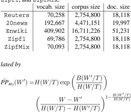
Theorem 7. For any distribution p′ on the LDA model withT topics learned from a corpusw′ re-duced from the original corpuswfollowing Zipf ’s law, assuming that each document only has one topic which is assigned based on a discrete uni-form distribution, the perplexity PPˆ Mix of theλ∗
calcu-Table 1: Details ofReuters,20news,Enwiki,
Zipf1, andZipfMix.
vocab. size corpus size doc. size
Reuters 70,258 2,754,800 18,118
20news 192,667 4,471,151 19,997
Enwiki 409,902 16,711,226 51,231
Zipf1 69,786 2,754,800 18,118
ZipfMix 70,093 2,754,800 18,118
lated by
ˆ
PPMix(W′) =H(W/T) exp (
B(W′/T)
H(W/T)
)
(
W −W′
H(W/T)−H(W′/T)
)1−H(W′/T)
H(W/T)
Proof. We can prove this by using a similar
argu-ment to that of Theorem 3 for each topic.
The formula of the theorem is nearly identical to the one of Theorem 3 for a 1/T corpus. This implies that the growth rate of the perplexity of LDA models is larger than that of unigram mod-els, whereas the perplexity of LDA models for the original corpus is smaller than that of unigram models. In fact, a similar argument to the one in the approximate analysis in Section 3.1 leads to an approximate formulaPP˜ MixofPPˆ Mixas
˜
PPMix(W′) = √
W T ln
W T exp
(lnW′−lnW)2
2 ln (W/T) ,
when W is sufficiently large. That is,PP˜ Mix(W′)
also has a quadratic behavior in a log-log graph, i.e.,PP˜ Mix(W′) =O(W′lnW
′ ).
4 Experiments
We performed experiments on three real corpora (Reuters,20news, and Enwiki) and two syn-thetic corpora (Zipf1 and ZipfMix) to verify the correctness of our theory and to examine the gap between theory and practice. Reuters and
20news here denote corpora extracted from the Reuters-21578 and 20 Newsgroups data sets, re-spectively. Enwikiis a1/100corpus of the En-glish Wikipedia.Zipf1is a synthetic corpus gen-erated by Zipf’s law, whose corpus is the same size asReuters, andZipfMixis a mixture of 20 syn-thetic corpora, sizes are 1/20th of Reuters. We usedZipfMix only for the experiments on topic models. Table 1 lists the details of all five corpora.
Fig. 1(a) shows the word frequency of
Reuters, 20news,Enwiki, andZipf1versus
frequency ranking on a log-log graph. In all cor-pora, we can regard each curve as linear with a gradient close to 1. This means that all corpora roughly follow Zipf’s law. Furthermore, since the curve of Zipf1 is similar to that of Reuters,
Zipf1can be regarded as acceptable.
Fig. 1(b) plots the perplexity of unigram mod-els learned from Reuters, 20news, Enwiki, and Zipf1 versus the size of reduced vocabu-lary on a log-log graph. Each value is the aver-age over different test sets of five-fold cross val-idation. Theory1 is calculated using the for-mula in Theorem 3. The graph shows that the curve of Theory1 is nearly identical to that of
Zipf1. Since the vocabulary sizeWτ of each test set is small in this experiment, some errors appear when W′ is large, i.e., Wτ < W′. This clearly means that our theory is theoretically correct for an ideal corpusZipf1. ComparingZipf1with
Reuters, however, we find that their perplex-ities are quite different. The reason is that the gap between the frequencies of low-ranking (high-frequency) words is considerably large. For ex-ample, the frequency of the 1st-rank word of
Reuters is f(w) = 136,371, while that of
Zipf1isf(w) = 234,705. Our theory seems to be suited for inferring the growth rate of perplexity rather than the perplexity value itself.
As for the approximate formula PP˜ 1 of Theo-rem 3, we can surely regard the curve ofZipf1
as being roughly quadratic. The curves of real corpora also have a similar tendency, although their gradients are slightly steeper. This difference might have been caused by the above-mentioned errors. However, at least, we can ascertain the important fact that the results for the corpora re-duced by 1/100 are not so different from those of the original corpora from the perspective of their perplexity measures.
Fig. 1(c) plots the frequency of k-grams (k ∈
{1,2,3}) in Reuters versus frequency ranking on a log-log graph.TheoryFreq(1-3) are calcu-lated usingCk in Lemma 4 andπk in Lemma 5. A comparison ofTheoryFreqandZipfverifies the correctness of our theory. However, comparing
[image:7.595.71.296.91.282.2]se-100 101 102 103 104 105 106
Frequency Ranking
100
101
102
103
104
105
106
107
Frequency
Reuters 20news Enwiki Zipf1
(a) Frequency of unigrams
100 101 102 103 104 105 106
Reduced Vocabulary Size
103
104
105
Test-set Perplexity
Reuters 20news Enwiki Zipf1 Theory1
(b) Perplexity of unigram models
100 101 102 103 104 105
Frequency Ranking
101
102
103
104
105
Frequency
Reuters Zipf1 TheoryFreq1 Reuters2 Zipf2 TheoryFreq2 Reuters3 Zipf3 TheoryFreq3
(c) Frequency ofk-grams
1 2 3 4 Gram Size5 6 7 8 9 10 0.4
0.6 0.8 1.0 1.2
Ex
po
ne
nt
Reuters TheoryExp
(d) Exponent of a power law overk -grams
100 101 102 103 104 105 106 107
Reduced Vocabulary Size
102
103
104
105
106
Te
st
-s
et
P
er
pl
ex
it
y
Reuters Zipf1 Theory1 Reuters2 Zipf2 Theory2 Reuters3 Zipf3 Theory3
(e) Perplexity ofk-gram models
100 101 102 103 104 105 106
Reduced Vocabulary Size
103
104
105
Te
st
-s
et
P
er
pl
ex
it
y
Reuters 20news Enwiki Zipf1 Theory1 ZipfMix TheoryMix TheoryAve
(f) Perplexity of topic models
Figure 1: (a) Word frequency ofReuters,20news, Enwiki, andZipf1versus frequency ranking. (b) Perplexity of unigram models learned fromReuters,20news,Enwiki, andZipf1versus size of reduced vocabulary. Theory1is calculated using the formula in Theorem 3. (c) Frequency ofk-grams (k∈ {1,2,3}) inReutersandZipf1versus frequency ranking. The suffix digit of each label means its gram size.TheoryFreq(1-3) are calculated using Lemma 4 and Lemma 5. (d) Exponent of a power law overk-grams inReutersversus gram size. TheoryGradis calculated usingπkin Lemma 5. (e) Perplexity ofk-gram models learned fromReutersversus size of reduced vocabulary. Theory2and
Theory3 are calculated using the formula in Corollary 6. (f) Perplexity of topic models learned from
Reuters,20news,Enwiki,Zipf1, andZipfMixversus size of reduced vocabulary.TheoryMixis calculated using the formula in Theorem 7.
quences in our simple model. The frequencies of high-orderk-grams tend to be lower than in real-ity. We might need to place a hierarchical assump-tion on the a power law, as in done in hierarchical Pitman-Yor processes (Wood et al., 2011).
Fig. 1(d) plots the exponent of the power law over k-grams in Reuters versus the gram size on a normal graph. We estimated each exponent of Reuters by using the least-squares method.
TheoryGradis calculated usingπkin Lemma 5. Surprisingly, the real exponents of Reuters are almost the same as the theoretical estimate πk based on our “stupid” model that does not care about the order of words. Note that we do not use any information other than the vocabulary sizeW and the gram sizekfor estimatingπk.
Fig. 1(e) plots the perplexity of k-gram mod-els (k ∈ {1,2,3}) learned fromReutersversus the size of reduced vocabulary on a log-log graph.
Theory2andTheory3 are calculated using the formula in Corollary 6. In the case of bigrams, the perplexities ofTheory2are almost the same as that ofZipf2when the size of reduced vocab-ulary is large. However, in the case of trigrams, the perplexities ofTheory3are far from those of
Zipf3. This difference may be due to the sparse-ness of trigrams inZipf3. To verify the correct-ness of our theory for higher orderk-gram models, we need to make assumptions that include backoff and smoothing.
Fig. 1(f) plots the perplexity of LDA models with 20 topics learned from Reuters, 20news,
Enwiki,Zipf1, andZipfMixversus the size of reduced vocabulary on a log-log graph. We used a collapsed Gibbs sampler with 100 iterations to infer the parameters and set the hyper parameters,
[image:8.595.77.521.60.325.2]distribu-Table 2: Computational time and memory size for LDA learning on the original corpus, (1/10)-reduced corpus, and (1/20)-(1/10)-reduced corpus of
Reuters.
corpus time memory perplexity original 4m3.80s 71,548KB 500
(1/10) 3m55.70s 46,648KB 550 (1/20) 3m42.63s 34,024KB 611
tionθˆdby using the first half of each test document and calculated the perplexity on the second half, as is done in (Asuncion et al., 2009). Each value is the average over different test sets of five-fold cross validation. Theory1 and TheoryMix
are calculated using the formulae in Theorem 3 and Theorem 7, respectively. Comparing Zipf1
withTheory1, andZipfMixwithTheoryMix,
we find that our theory of the extreme cases discussed in Section 3.3 is theoretically cor-rect. TheoryAve is the average of Theory1
and TheoryMix. Comparing Reuters and
TheoryAve, we see that their curves are almost the same. If theoretical perplexity PP has aˆ
similar tendency as real perplexity PP on a log-log graph, i.e., lnPP(W′) ≈ ln ˆPP(W′) +c
for some constant c, we can approximate its deterioration rate as PP(W′)/PP(W) ≈ exp (ln ˆPP(W′) +c)/exp (ln ˆPP(W) +c) =
ˆ
PP(W′)/PPˆ (W). Therefore, we can use
TheoryAve as a heuristic function for estimat-ing the perplexity of topic models. Since we can calculate an inverse of TheoryAve from the bisection or Newton-Raphson method, we can maximize the reduction rate and ensure an acceptable perplexity based on a user-specified deterioration rate. According to the fact that the three real corpora with different sizes have a similar tendency, it is expected that we can use our theory for a larger corpus.
Finally, let us examine the computational costs for LDA learning. Table 2 shows computa-tional time and memory size for LDA learning on the original corpus, (1/10)-reduced corpus, and (1/20)-reduced corpus of Reuters. Comparing the memory used in the learning with the origi-nal corpus and with the (1/10)-reduced corpus of
Reuters, we find that the learning on the (1/10)-reduced corpus used 60% of the memory used by the learning on the original corpus. While the computational time decreased a little, we believe that reducing the memory size helps to reduce
computational time for a larger corpus in the sense that it can relax the constraint for in-memory com-puting. Although we did not examine the accuracy of real tasks in this paper, there is an interesting report that the word error rate of language mod-els follows a power law with respect to perplexity (Klakow and Peters, 2002). Thus, we conjecture that the word error rate also has a similar tendency as perplexity with respect to the reduced vocabu-lary size.
5 Conclusion
We studied the relationship between perplexity and vocabulary size of reduced corpora. We de-rived trade-off formulae for the perplexity of k -gram models and topic models with respect to the size of reduced vocabulary and showed that each formula approximately has a simple behavior on a log-log graph under certain conditions. We veri-fied the correctness of our theory on synthetic cor-pora and examined the gap between theory and practice on real corpora. We found that the es-timation of the perplexity growth rate is reason-able. This means that we can maximize the reduc-tion rate, thereby ensuring an acceptable perplex-ity based on a user-specified deterioration rate. Furthermore, this suggests the possibility that we can theoretically derive empirical parameters, or “rules of thumb”, for different NLP problems, as-suming that a corpus follows Zipf’s law. We be-lieve that our theoretical estimation has the advan-tages of computational efficiency and scalability especially for very large corpora, although exper-imental estimations such as cross-validation may be more accurate.
In the future, we want to find out the cause of the gap between theory and practice and extend our theory to bridge the gap, in the same way that we can construct equations of motion with air re-sistance in the example of the landing point of a ball in Section 1. For example, promising re-search directions include using a general law such as the Zipf-Mandelbrot law (Mandelbrot, 1965), a sophisticated model that cares the order of words such as hierarchical Pitman-Yor processes (Wood et al., 2011), and smoothing/backoff methods to handle the sparseness problem.
Acknowledgments
References
Arthur Asuncion, Max Welling, Padhraic Smyth, and Yee Whye Teh. 2009. On smoothing and infer-ence for topic models. In Proceedings of the 25th
Conference on Uncertainty in Artificial Intelligence (UAI2009), pages 27–34. AUAI Press.
Ioannis Atsonios, Olivier Beaumont, Nicolas Hanusse, and Yusik Kim. 2011. On power-law distributed balls in bins and its applications to view size esti-mation. In Proceedings of the 22nd International
Symposium on Algorithms and Computation (ISAAC 2011), pages 504–513. Springer-Verlag.
David M. Blei, Andrew Y. Ng, and Michael I. Jordan. 2003. Latent Dirichlet Allocation. Journal of
Ma-chine Learning Research, 3:993–1022.
Shahar Boneh and Vassilis G. Papanicolaou. 1996.
General asymptotic estimates for the coupon collec-tor problem. Journal of Computational and Applied
Mathematics, 67(2):277–289.
Thorsten Brants, Ashok C. Popat, Peng Xu, Franz J.
Och, and Jeffrey Dean. 2007. Large Language
Models in Machine Translation. In Joint
Confer-ence on Empirical Methods in Natural Language Processing and Computational Natural Language Learning (EMNLP-CoNLL2007), pages 858–867.
ACL.
Adam L. Buchsbaum, Raffaele Giancarlo, and
Jef-fery R. Westbrook. 1998. Shrinking Language
Models by Robust Approximation. In
Proceed-ings of the 1998 IEEE International Conference on Acoustics, Speech and Signal Processing (ICASSP 1998), pages 685–688.
Stanley F. Chen and Joshua Goodman. 1996. An em-pirical study of smoothing techniques for language modeling. In Proceedings of the 34th annual
meet-ing on Association for Computational Lmeet-inguistics (ACL 1996), pages 310–318. ACL.
Ken Church, Ted Hart, and Jianfeng Gao. 2007. Com-pressing Trigram Language Models with Golomb Coding. In Joint Conference on Empirical
Meth-ods in Natural Language Processing and Computa-tional Natural Language Learning (EMNLP-CoNLL 2007), pages 199–207. ACL.
Aaron Clauset, Cosma Rohilla Shalizi, and M. E. J. Newman. 2009. Power-Law Distributions in Em-pirical Data. SIAM Review, 51(4):661–703.
Jianfeng Gao and Min Zhang. 2002. Improving Lan-guage Model Size Reduction using Better Pruning Criteria. In Proceedings of the 40th Annual
Meet-ing of the Association for Computational LMeet-inguistics (ACL 2002), pages 176–182. ACL.
Sharon Goldwater, Thomas L. Griffiths, and Mark
Johnson. 2011. Producing Power-Law
Distribu-tions and Damping Word Frequencies with Two-Stage Language Models. Journal of Machine
Learn-ing Research, 12:2335–2382.
Joshua Goodman and Jianfeng Gao. 2000.
Lan-guage Model Size Reduction by Pruning and
Clus-tering. In Proceedings of the 6th International
Conference on Spoken Language Processing (ICSLP 2000), pages 110–113. ISCA.
Thomas L. Griffiths and Mark Steyvers. 2004. Find-ing scientific topics. In ProceedFind-ings of the National
Academy of Sciences of the United States of America (PNAS 2004), volume 101, pages 5228–5235.
Le Quan Ha, E. I. Sicilia-Garcia, Ji Ming, and F. J. Smith. 2002. Extension of Zipf’s Law to Words and Phrases. In Proceedings of the 19th International
Conference on Computational Linguistics (COLING 2002), pages 1–6. ACL.
Le Quan Ha, P. Hanna, D. W. Stewart, and F. J. Smith. 2006. Reduced n-gram models for English and Chi-nese corpora. In Proceedings of the 21st
Interna-tional Conference on ComputaInterna-tional Linguistics and 44th Annual Meeting of the Association for Compu-tational Linguistics, Proceedings of the Conference (COLING-ACL 2006), pages 309–315. ACL.
Teemu Hirsimaki. 2007. On Compressing N-Gram Language Models. In Proceedings of the 2007 IEEE
International Conference on Acoustics, Speech and Signal Processing (ICASSP 2007), pages 949–952.
Dietrich Klakow and Jochen Peters. 2002. Testing the correlation of word error rate and perplexity. Speech
Communication, 38(1):19–28.
Hailong Li. 2005. On Generalized Euler Constants and an Integral Related to the Piltz Divisor Problem.
˘
Siauliai Mathematical Seminar, 8:81–93.
Benoit B. Mandelbrot. 1965. Information Theory
and Psycholinguistics: A Theory of Word Frequen-cies. In Scientific Psychology: Principles and
Ap-proaches. Basic Books.
OEIS. 2001. The on-line encyclopedia of
inte-ger sequences (a061017). http://oeis.org/
A061017/.
Mark Steyvers and Tom Griffiths. 2007. Probabilis-tic Topic Models. In Handbook of Latent SemanProbabilis-tic
Analysis, pages 424–440. Lawrence Erlbaum
Asso-ciates.
Andreas Stolcke. 1998. Entropy-based Pruning of
Backoff Language Models. In Proceedings of the
DARPA Broadcast News Transcription and Under-standing Workshop, pages 270–274.
Frank Wood, Jan Gasthaus, C´edric Archambeau, Lancelot James, and Yee Whye Teh. 2011. The Se-quence Memoizer. Communications of the
Associa-tion for Computing Machines, 54(2):91–98.
George Kingsley Zipf. 1935. The Psychobiology of