Trade and Environment: Do Spatial
Effects Matter?
Azam, Sardor
February 2016
Online at
https://mpra.ub.uni-muenchen.de/73113/
JAEBR, 6 (2): 161-174 (2016)
Trade and Environment: Do Spatial Effects Matter?
Sardor Azam
1Institute of Forecasting and Macroeconomic Research, Tashkent, Uzbekistan Westminster International University in Tashkent, Tashkent, Uzbekistan
Abstract
This study tests the suitability of spatial effects in trade context. The paper analyzes the effect of the strictness of environmental regulations on trade performance on the basis of augmented gravity model. It compares spatial estimates with those of OLS and concludes that spatial effects are important. The results indicate that Spatial Error Model fits best to the data at hand. It is shown that environmental standards are positively correlated with trade.
Keywords: Exports, Augmented gravity model, Environmental Performance Index, Spatial econometrics, Multilateral resistance
JEL Classification: C31, F18, Q56
Copyright © 2016 JAEBR
1. Introduction
Environmental and trade linkage has become an issue of academic and research scrutiny starting from late 1960s and early 1970s. Since then many questions have been raised and applied to empirical tests. One of the major questions that needed to be answered has been whether the stringency of environmental regulations negatively affects the country’s foreign trade and especially its exports. The answer to the question has been of major importance to the theory of international trade as well. Diverse empirical results have been taken so far. At the same time, related estimation methodology and analytical techniques have been developed to deal with this and more general economic issues.
Theoretically it has been believed that the stricter the environmental regulations are the more international competitiveness the domestic industries suffer. This is because stringent regulations exert some sort of pressure on domestic polluters to take abatement activities, which increases production costs and thus deteriorates competitiveness. Eventually these firms move their production abroad to developing countries where economic development issues are generally regarded as more important than environmental problems. As a result, the country loses its exports markets in these sectors, but starts importing products of polluting industries from overseas markets. This process has become known as “pollution-haven hypothesis” in the environmental literature.
It can be pointed out that the pollution-haven hypothesis changes the patterns of international trade. Developed countries become more specialized in producing environmentally-friendly products while developing ones become more inclined to produce pollution-intensive goods. However, sometimes strict domestic environmental policies in developed countries impose restrictions in
importing products of polluting industries from abroad. This causes bipolarization of trade in such goods among countries.
So far there have been numerous attempts to test empirical grounds for such theoretical conclusions. Based on the review of retrospective literature on the topic, Cropper and Oates (1992) try to look into the extent environmental measures had influenced the pattern of international trade before 1992. Referring to major papers in the area, they conclude that the stringency of domestic environmental policies hadn’t had any significant effect on trade patterns. The reason they suggest might have been negligibly lower costs of pollution control in pollution-intensive sectors by then.
Xu (2000) analyzes the effect of stringent domestic environmental policies on international competitiveness of environmentally sensitive goods (ESGs) using cross-sectional data from 20 countries in 1990. Employing time-series tests for systematic changes in countries that introduced environmental stringency measures and based on the results of extended gravity model approach, he confirms most of previous results in the area that more stringent environmental regulations do not reduce total exports, exports of ESGs and exports of non-resource-based ESGs. The researcher also finds no evidence of trade barriers arisen from introduction of more stringent environmental regulations by foreign countries.
However, a different conclusion was suggested by Porter and Linde (1995). They show that despite short-run losses, in the long-run a country with stricter environmental regulations is likely to nurture new comparative advantages in the environmentally more sensitive sectors. They believe that this helps to create a new trade pattern for the country.
One of the most influential papers on the area is one by Beers and Bergh (1997). They attribute the inconclusiveness of previous research results to the usage of improper variables in representing the strictness of environmental policies. They test two measures of stringency in a gravity model framework using 1992 data for all OECD member-countries. After performing the analysis for total trade, pollution-intensive trade (“dirty”), and pollution-intensive trade related to non-resource-based (“footloose”) industries, respectively, the authors conclude that the closer the environmental policy strictness measure to the Polluter Pays Principle is, the more conclusive the estimates will become. Based on the narrow measure they use to represent the stringency of environmental regulations, their findings reveal the following:
a) The empirical test of total and “footloose” trade structures shows that a more stringent environmental policy has a significant negative impact on exports while such an impact cannot be observed in pollution-intensive exports. This indicates that existence or an ease of access to the natural resources in a country exerts higher influence on determining the competitiveness of pollution-intensive “footloose” industries than environmental standards.
b) It turns out that stringent environmental regulations are negatively correlated with all three types of imports (aggregate, “dirty”, and “footloose”). This indicates that countries with stringent environmental policies also carry out import-substitution trade policy through imposing non-tariff barriers on imports from abroad.
Costantini and Crespi (2008) have suggested the opposite result to what Beers and Bergh (1997) and some other studies have found. They test an empirical model based on a gravity equation to provide empirical evidence for the Porter and Linde hypothesis. Their conclusion is that “a more stringent environmental regulation provides a positive impulse for increasing investments in advanced technological equipment, thus providing an indirect source of comparative advantages at international level. Countries with stringent environmental standards have a higher export capacity for those environmental-friendly technologies that regulation induces to adopt” (Constantini and Crespi, 2008).
As is seen, all of these studies have so far come up with different results. Some researchers attributed this to the usage of inappropriate proxies for strictness of environmental regulations variable due to a lack of adequate and reliable data on it, the fact that was mentioned above. In measuring the stringency of environmental regulations variable one should take into consideration the effects caused by governmental subsidies to pollution-intensive industries, environmental standards that imported products face, industry location issues such as proximity and ease of access to natural resources and markets, the supply and quality of labor, transportation costs etc. It may be a case that the effect of these economic fundamentals may outweigh that of environmental cost factors.
Sometimes it is the usage of inappropriate modeling and estimation techniques that may cause inconclusive results. So far most analyses use either the gravity model or the Heckscher-Ohlin-Vanek (HOV) factor endowment model to study the effect of environmental regulations on trade competitiveness.
Research papers by Tobey (1990), Cole and Elliott (2003), and Babool and Reed (2010) utilize HOV model. For instance, a study by Babool and Reed (2010) follows the standard factor endowment approach to explain the effects of environmental regulatory policy on net exports in different product-based industries. Their results indicate that each industry has unique characteristics in the factors determining its net exports and in many cases environmental regulations are important. Using a panel dataset of 10 OECD countries over 17 years (1987-2003), they find a positive relationship between net exports and environmental regulations in such industries as paper production, wood production and textile production.
In this paper we undertake an empirical test of the hypothesis that countries with stringent environmental regulations face lower levels of exports and higher levels of imports. We argue that testing for spatial effects in gravity models is a necessary part of studying such issues as the environmental regulations and trade linkage that may carry unobserved geographical (spatial) information. Although we were not able to construct panel data framework to study the issue, which would be our future goal, we believe that our results would still bring fresh air in the estimation part of the area under concern.
2. Model
2.1. Augmented gravity model component
In general, gravity models have been widely used by trade economists for the last half a century to measure international trade and investment flows between countries. The origin of the gravity equation as a tool for measuring and modeling bilateral trade flows between countries is “intuitive approximation, not a hypothetical deductive” (Sanso et al., 1993). Despite its lack of strong theoretical foundation, the gravity model has exhibited sound explanatory power and empirical robustness. In particular, its appeal is based on its ability to explain the real phenomena in international trade that are consistent with factor endowment, technological differences theories, increasing returns to scale, and “Armington” demands models. However, within the gravity model frameworks most recent studies focus on estimating the effects of economic-integration-type of issues, such as regional trade agreements, currency unions, common markets, etc., and their role in creating or diverting trade.
The basic theoretical model of gravity for trade is taken from Newtonian law of gravity and can be expressed in the stochastic form as follows:
where: TRADEij is trade flows (can be exports or imports as well) from country i to country j; A is a constant term; GDP is a current value of income (output) in country i and j depending on
subscript; DISTij is distance between i and j; uij is a normal random error term; and β β β1, 2, 3 are
parameters. I.e. the equation states that the trade flows between involved countries, TRADEij, is proportional to the product of the two countries’ GDPs, and inversely proportional to their distance, Dij, to account for all possible factors that might create trade resistance.
A model specification is an important issue in gravity model context. In many cases different variables which are of crucial relevance to either an exporter or importer countries should be included into the basic theoretical model. Those can be area size, GDP per capita along with GDP, common language (dummy), membership to different Free Trade Areas (FTAs) or trade organizations or geographical regions (dummy), common border or border type [sea or land] (dummy), colony or colonizer (dummy), bilateral exchange rate, tariffs, trade complementarity (index), etc. Without proper specification there is no doubt that the estimates can be biased and inconsistent. For example, Kalirajan (2008) notes that the economic distance between country i and j is often replaced by geographical distance that can lead to biased estimates. Citing from Roemer (1977), he argues that “economic distance includes not only geographical distance, but also other country-specific factors such as historical and cultural ties between countries, the tying up of aid and the lines of communication between countries, which influence the intensity of trade between pairs of countries” (Kalirajan, 2008). One important point in here is that researchers should specify their models based upon not only universal variables that constitute the basis of gravity models, but also country-specific factors.
Along with other relevant variables, in the present context we augment traditional gravity equation to include strictness of environmental policy variables:
0 1 2 3 4
5 6 7 8 9
10 11
ln ln ln ln ln
ln
ln ln ,
ij i j i j
ij ij ij ij ij
i j ij
EX GDP GDP POP POP
DIST LNG BRD APEC SEA
EPI EPI
β β β β β
β β β β β
β β ε
= + + + + + + + + + + + + + + 1 2 3 *
* i j *
ij ij
ij
GDP GDP
TRADE A u
DIST
β β
β
where: ln denotes natural logarithm; EXij, the exports of country i to country j; GDPi, GDPj, the GDPs of countries i and j, respectively; POPi, POPj, the populations of countries i and j, respectively; DISTij, the distance between countries i and j; LNGij, BRDij, APECij, SEAij, dummy variables, equal to 1 if countries i and j share the same official language, share a common land border, are members of Asia-Pacific Economic Cooperation (APEC), have direct access to sea, respectively, and zero otherwise; EPIi, EPIj, Environmental Performance Indices representing the relative
strictness of environmental regulations in countries i and j, respectively; and ɛij, white noise
disturbance term.
In this model, β β1, 2 coefficients are expected to be positive since the higher the GDP of
exporter/importer countries, the higher the supply/demand of/for exports/imports will be. The coefficients of population are generally believed to be positive: for example, the higher the population of an importer country, the more imports it will be willing to accept, other things equal; the higher the population of an exporter country, the higher it may export because of economies of scale that it may benefit from. But it may also a case that exporter country with higher population may export less because of self-reliance behavior, that is, relative importance of domestic consumption. This is why the coefficient of POPi can be regarded as ambiguous. A slope parameter of DISTij is expected to be negative because it is a proxy that represents economic distance between countries, i.e. a term that captures trade resistance. The coefficients for all dummy variables included into the model, from LNGij to SEAij, are anticipated to be positive. The reason for this is that if, say, two trading partners share the same language (LNGij=1), then it is likely that the exporter may easily explore the market of trade partner and will export more goods to that country than to other countries.
We augment our gravity model with EPIi and EPIj variables that represent the degree of strictness of the environmental regulations in the exporter and importer countries, respectively. The data belong to the family of index numbers, with the larger number indicating high stringency of
environmental policy. We expect β10 to be negative and β11 to be positive since this is what our
earlier hypothesis suggests: relatively strict domestic environmental regulations result in lower
exports and higher imports. At the same time, one should not forget that if β10 turns out to be positive,
then that means exporter countries have a comparative advantage in the environmentally more
sensitive industries. By the same token, β11 coefficient may empirically turn out to be negative, which
suggests that importer countries defend their domestic “dirty” industries from foreign competition by
imposing trade barriers for imports and/or through subsidizing them. In brief, the signs of β10 and
11
β
are ambiguous.
2.2. Spatial effects component
Now when we constructed augmented gravity model with hypothetical expectations about its coefficients, we should turn to the justification of incorporating spatial effects into it. Actually it may well be a case that spatial effects are statistically insignificant, in which situation the estimation of augmented gravity model with OLS will suffice.
among themselves. They may have some kind of dependence in all directions and it becomes weaker as data locations become more and more dispersed. Tobler’s “First Law of Geography” (Tobler, 1979) says: “Everything is related to everything else, but near things are more related than distant things.” Spatial autocorrelation can be positive or negative. Positive spatial autocorrelation occurs when similar values occur near one another. Negative spatial autocorrelation occurs when dissimilar values occur near one another.
To account for that relationship, whether it is close or distant, relative spatial positions are represented by spatial weights matrices (W-matrix). There are different types of those matrices that can be constructed. For instance, econometricians usually use inverse distance weights matrices where essentially neighborhood relationships are stronger the closer the points are to each other.
The values observed at one location can depend upon values in other neighboring locations where W-matrices serve as strength of a link. The sum of values in neighboring locations is called a spatial lag. The general expression for the spatial lag or spatial autoregressive model (SAR) is presented here:
2
~ (0, ),
y Wy X
N I
ρ β ε
ε σ
= + +
where y is nx1 vector of dependent variable observations; Wy is nx1 vector of lagged dependent
variable observations; ρ is a spatial autoregressive parameter; X is an nxk matrix of explanatory
variables; β is a kx1 vector of respective coefficients; and ε is an nx1 vector of independent
disturbance terms.
Moving all terms that have the dependent variable y to the left-hand side and subsequent manipulations will result in the following expressions:
1 1
( )
( ) ( ) ,
I W y X
y I W X I W
ρ β ε
ρ − β ρ − ε
− = +
= − + −
where
1
(I−ρW)− is called a spatial multiplier term. This term tells us how much of the change
in Xi will “spill over” onto other countries j and in turn affect yi through the impact of y in the spatial lag. Since both a matrix of independent variables and error term have the same spatial multiplier term that now becomes part of them, independent variables and error term are correlated, a fact that violates Gauss-Markov theorem. This is why OLS estimation of such a simultaneity situation caused by endogeneity will result in biased estimates. Since this may be a case, mainly Maximum Likelihood Estimation and Instrumental Variables techniques are used to analyze and estimate spatial econometric regression models. In spatially lagged y models MLE is consistent and asymptotically
efficient if the model is correctly specified. One should note that in case if ρ =0, then OLS estimates
are also BLUE.
Another wide-spread model in spatial analysis is spatial error model (SEM). In this case spatial dependence enters through the error terms rather than through the systematic component of the model. The observations are related only due to unmeasured factors that, for some unknown reason, are correlated across distances among the observations. The representation of SEM model stems from the following:
2
,
,
~ (0, )
y X u
Manipulating the error term yields:
1
( ) ,
( )
I W u
u I W
ρ ε
ρ −ε
− =
= −
Finally, the basic data generating process for SEM model is shown here:
1 2
( ) ,
~ (0, )
y X I W
N I
β ρ ε
ε σ
−
= + −
If systematic component of the model is correctly specified and there is still some correlation in the error terms, it is useful to employ SEM to correct for this problem in the residual since it provides a substantial improvement of the model.
Generally speaking, gravity models in trade are one of common areas where SEM models are appropriate. Anderson and Wincoop (2003) argue that dealing with the regional interactions is vital when dealing with gravity models. In trade models such as this so called “multilateral resistance” terms, which “capture the fact that bilateral trade flows do not only depend on bilateral trade barriers but also on trade barriers across all trading partners” (Behrens et al., 2012), are usually reflected in spatial error structure. Multilateral resistance terms are very important concept in this context simply due to the fact that nowadays most of intermediate products cross many borders to get manufactured in the form of a final good and reach the final consumer. Vertical specialization patterns make it important to consider trade barriers across these borders.
In order to see which spatial model is suitable to our dataset, we carry out robustness tests described in greater detail in Section 5. Since spatial relationships in the data violate the assumptions underlying OLS leading either to inefficiency and invalid hypothesis testing procedures in the case of spatial error dependence, or to bias and inconsistent parameter estimates in the case of spatial regression and spatial lags, we present a comparison of OLS estimates versus spatial estimates in the that section.
3. Data
We use a cross-sectional dataset where dependent variable is exports of China with its 40 main trading partners in 2009 (see Appendix A for countries included, Taiwan is excluded due to lack of data). 30% of countries under the study are developed countries. Since our dataset also involves trade relations of all these countries with each other (not only bilateral trade of China), it doesn’t make any sense to claim that we study only China’s exports. The reason for selection of such a dataset is that we initially used it for a different econometric purpose. Here we argue that the selection of countries doesn’t affect the results because it can be treated as a random selection. Although many papers mainly use data from member-countries of OECD-like structures, yet some other papers select them randomly (e.g., Xu, 2000).
Sources of data are IMF Direction of Trade Statistics for export data; IMF World Economic Outlook data for real GDP, GDP deflator, and population of all countries including China; data from
www.itouchmap.com on longitude and latitude of each capital city of the countries under the study to construct distance parameter in the W-matrix; Environmental Performance Index that represents
the stringency of environmental standards is taken from the archive of epi.yale.edu. The values of
dummies are input by the author based on publicly available information.
with logarithms, we input USD 0.01 mln or USD 10,000 for each of such zero trade cases to avoid selection bias and keep trade among such countries in the dataset. For observations when each country trades with itself (Behrens et al., 2012) call it “domestic consumption”), we calculated it as GDP minus total exports of a country. All non-dummy variables such as exports, real GDP of importer and exporter countries, and importer and exporter population are in millions of USD. Distance is in thousands of kilometers.
Overall, our dataset consists of 1600 observations (40x40). We used GAUSS 11.0 econometric package to perform our calculations.
3.1. Environmental Regulations Indicator
One of the weakest points in the research papers on the current topic is that it is difficult to find an appropriate proxy for the strictness of environmental regulations indicator. Many empirical findings are questioned because the studies lack adequate and reliable data on environmental regulations. To solve the problem, studies end up using either environmental regulation indices or data collected by surveys. Hereby we provide a brief literature review on this issue and justify our way of dealing with the problem.
Beers and Bergh (1997) prefer using output-oriented indicators that can be considered as a better proxy than input-oriented indicators under the assumption that better environmental performance is due to stricter environmental regulations. Using output-oriented indicators, they construct an environmental regulations strictness measure that is closely consistent with the Polluter Pays Principle.
In Harris et al. (2002) the stringency of environmental regulations is measured by six different indicators, all of which are based on either the relative energy consumption or on relative energy supply.
Xu (2000) makes use of a set of unique environmental stringency indices developed by the World Bank in 1995. Since this survey draws information on the state of policy and performance in four environmental dimensions, namely, air, water, land and living resources, the resulting composite environmental stringency index, as the author is convinced, can serve as a good proxy for environmental stringency.
A relatively new approach is pursued by Soest et al. (2006). They develop a method to measure environmental stringency by estimating a shadow price for a polluting input, the first attempt at providing such figures by using a standard neoclassical cost function approach.
Regarding the main linkages between environmental regulations and trade patterns, Busse (2004) uses two core indicators: environmental governance and participation in international cooperative efforts. The former is a composite indicator that is comprised of such measures as the ratio of petrol price to international average, World Economic Forum survey questions on environmental governance, the percentage of land area under protected status, the number of sector environmental impact assessment guidelines, 7 accredited forest area as a percentage of total forest area, measures of corruption, the World Economic Forum subsidies survey question, and the WWF (World Wide Fund for Nature) subsidy measure. The authors believe that this indicator provides a comprehensive measure of the stringency of environmental regulations across countries.
indicators provide a gauge at a national government scale of how close countries are to established environmental policy goals. The higher the EPI score is, the stricter the environmental regulations are. We believe that this set of indices encompasses many aspects of environmental policy and therefore can be used as a good proxy variable for environmental stringency. Internal indicators that the EPI is constructed from are listed in Appendix B or can be found in epi.yale.edu/downloads.
4. Estimation Results and Discussion
In this section we discuss the W-matrix we use, indicate our estimation method, show the results we get, and interpret stringency indicators.
Generally, in order to estimate spatial autocorrelation, one first needs to define what is meant by two observations being close together, i.e., a distance measure must be determined. These distances are presented in W-matrix, which defines the relationships between locations where measurements were made. If data are collected at n locations, then the W-matrix will be nxn with zeroes on the diagonal.
The W-matrix can be specified in many ways: (a) the weight for any two different locations can be a constant; (b) all observations within a specified distance can have a fixed weight; (c) K nearest neighbors can have a fixed weight, and all others are zero (contiguity W-matrices); (d) weight can be proportional to inverse distance, inverse distance squared, or inverse distance up to a specified distance. Literature shows that other W-matrices are also possible.
In our model, along with generally accepted distance variable, we also use importer population variable to capture the effects of population in trade. While distance variable is used to measure how distance influences trade (the farther the distance between trading countries is, the less trade will occur), importer population variable is used to test how population affects trade (the more the population of an importer country is, the more trade will likely be observed). Among the W-matrix family we find that contiguity W-matrix is suitable in our context since it gives decent results. However, the results were still consistent when we experimented with other specifications (matrices) of W, an indication that confirms we don’t have any misspecification problem in the model.
Generally, spatial models are econometrically estimated with maximum likelihood estimation (MLE) method, generalized method of moments (GMM), or instrumental variable (IV) method. Since GMM is more general technique and has decent properties in terms of efficiency and consistency in large samples, we use this method in our estimations.
Table 1. Testing for spatial effects
Case I: Distance as weight
TESTS Chi-sq Prob > Chi-sq
Breusch-Pagan-White (SEM) 114.23 1.5693e-025
LM (SEM) 45.612 1.4415e-011
Robust LM (SEM) 29.795 4.8032e-008
Moran’s I (SAR) 0.039 6.9059e-015
LM (SAR) 17.682 2.6115e-005
Robust LM (SAR) 1.8641 0.17215
Case II: Importer population as weight
TESTS Chi-sq Prob > Chi-sq
Breusch-Pagan-White (SEM) 114.23 1.5693e-025
LM (SEM) 34.234 4.8865e-009
Robust LM (SEM) 25.150 5.3038e-007
Moran’s I (SAR) 0.058 4.9521e-011
LM (SAR) 11.340 0.00075849
Robust LM (SAR) 2.2561 0.13309
[image:11.595.81.554.481.748.2]The results indicate that in the first case, where distance is used as a weight in W-matrix, SEM model is appropriate. So our dataset indeed has spatial heterogeneity. Robust LM test for spatial dependence indicate that with the probability of 17% we can accept the null hypothesis of not having SAR model (so we don’t have it).
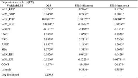
Table 2. Estimation results and robustness check
Dependent variable: ln(EX)
VARIABLES OLS SEM (distance) SEM (imp.pop.)
lnEX_GDP 0.9775* 0.9745* 0.9724*
lnIM_GDP 0.7450* 0.7435* 0.8091*
lnEX_POP 0.0002*** 0.0002*** 0.0004***
lnIM_POP 0.0004** 0.0004** 0.0005**
lnDIST -0.1916* -0.1922* -0.1933*
LNG 1.0968* 1.0590* 0.9979*
BRD 2.1829* 2.2119* 2.2306*
APEC 1.1337* 1.1834* 1.2613*
SEA 1.2759* 1.3129* 1.2678*
lnEX_EPI 0.0426* 0.0424* 0.0429*
lnIM_EPI 0.0206* 0.0223** 0.0174***
CONS -19.574* -19.559* -20.179*
Lambda --- 0.3831* 0.3899*
Log-likelihood -3270.5 --- ---
Almost similar conclusion can be made in the second case where importer population is used as a weight. At 5% level of significance we reject that the model has spatial lag structure. So even in this case SEM seems to be appropriate for modeling.
In Table 2 we present the results of estimation of spatial gravity model with SEM structure. To compare we also calculated OLS estimates of the gravity model with no spatial effects included.
As can be inferred from the table, the lambda coefficients for two SEM models are statistically significant even at 1% level. This is a verification that SEM model is indeed quite appropriate for the dataset at our hand. As can also be noticed, all coefficient estimates are very close to each other. In both cases where distance and importer population are used as weights for W-matrices, respectively, the estimates are stable. This is an indication that our model is correctly specified and the results are consistent. Individual t-statistics reveal that coefficients for GMM estimations of SEM models are more efficient than OLS estimates. At 5% level of significance the only difference between SEM models is that in the case where importer population is used as a weight the importer EPI index turns out to be statistically insignificant. Estimation results show that exporter population is not an important variable in our context.
Interpretation of estimation of EPI coefficients are as follows. At 5% level of significance and assuming that all other variables are kept constant, one percent increase in exporter EPI increases exports by 0.0424-0.0429%. By the same token, one percent increase in importer EPI increases exports by 0.0223% ceteris paribus at the same level of significance.
5. Conclusion
In this research paper we make an attempt to estimate the effects of the strictness of environmental regulations on exports based on augmented gravity model. The appropriateness of spatial effects in this context was scrutinized. We provide a brief introduction to spatial econometrics with examples of SEM and SAR models, and construct two W-matrices with distance and importer population as weights to check for spatial effects in a dataset of Chinese exports to 40 main export destination countries in 2009.
Our conclusion is that both domestic and foreign strictness of environmental regulations indicators have positive effects on trade. Since exporter EPI has such an effect, we may conclude that exporter countries have a comparative advantage in the environmentally more sensitive industries. This is why we find that “pollution-haven hypothesis” doesn’t hold in this context. This conclusion should be further checked because it might be a case that our dataset is biased towards including more developing countries (70%) rather than having an equal amount of both developed and developing countries. It may also be a case that developing countries don’t move their “dirty” industries into other less developed countries at least at this point of time. In the case where we use importer population as a weight accounting for interaction effects, we also find that importer EPI is statistically insignificant, which indicates that importer countries’ stringency of environmental regulations doesn’t matter. The estimation results show that exporter population is also statistically insignificant. Our tests for spatial heterogeneity and dependence find that spatial effects matter since they incorporate “multilateral resistance” that captures trade barriers not only among trading countries, but also their trade barriers across all trading partners. Thus, OLS estimation of augmented gravity model should be avoided. We conclude that SEM is the best choice to construct the spatial gravity model.
fluctuations”. Focusing on industry-based disaggregate level is also a good path to pursue. What might be more insightful is that we should test the relationship of different stringency variables, and if appropriate, construct a better proxy.
References
Anderson JE. 1979.A Theoretical Foundation for the Gravity Equation. American Economic Review
69, 106-16.
Anderson JE, van Wincoop E. 2003. Gravity with Gravitas: A Solution To The Border Puzzle.
American Economic Review 93:1, 171-92.
Anselin L. 1988. Spatial Econometrics: Methods and Models. Kluwer: Dordrecht, 284.
Anselin L. 2001. Spatial Effects in Econometric Practice in Environmental and Resource Economics.
American Journal of Agricultural Economics 83:3, 705-10.
Babool A, Reed M. 2010. The impact of environmental policy on international competitiveness in
manufacturing. Journal of Applied Economics 42, 2317-26.
Behrens K, Ertur C, Koch W. 2012. ‘Dual’gravity: Using spatial econometrics to control for
multilateral resistance. Journal of Applied Econometrics 27:5, 773-794.
Busse M. 2004. Trade, Environmental regulations and the World Trade Organization: New empirical
evidence. Journal of World Trade 38, 285-306.
Cole MA, Elliott RJR. 2003. Do Environmental Regulations Influence Trade Patterns? Testing Old
and New Trade Theories. The World Economy 26:8, 1163-86.
Cropper ML, Oates WE. 1992. Environmental Economics: A Survey. Journal of Economic Literature
30:2, 675-740.
Costantini V, Crespi F. 2008. Environmental Regulation and the Export Dynamics of Energy
Technologies. Ecological Economics 66:2-3, 447-60.
Environmental Performance Index, http://epi.yale.edu.
Ertur C, Koch W. 2007. Growth, Technological Interdependence and Spatial Externalities: Theory
and Evidence. Journal of Applied Econometrics 22, 1033-62.
Harris MN, Konya L, Matyas L. 2002. Modeling the Impact of Environmental Regulations on
Bilateral Trade Flows: OECD, 1990-1996. World Economics 25:3, 387-405.
IMF Direction of Trade Statistics, http://www.elibrary-data.imf.org.
IMF World Economic Outlook (WEO) data, http://www.econstats.com.
Jug J, Mirza D. 2005. Environmental Regulations in Gravity Equations: Evidence from Europe.
World Economics 28:11, 1591-1615.
Kalirajan K. 2008. Gravity Model Specification and Estimation: Revisited. Applied Economic Letters
15, 1037-39.
LeSage J, Pace K. 2009. Introduction to Spatial Econometrics, Taylor & Francis Group, LLC.
Lin K-P, lecture notes at WISE Xiamen University, China, Nov. 8-19, 2010 for “Spatial Econometric
Analysis Using Gauss” course [http://web.pdx.edu/~crkl/WISE/SEAUG.htm].
Lin K-P. 2001. Computational Econometrics: GAUSS Programming for Econometricians and
Longitude and latitude data on geographical points, http://www.itouchmap.com.
Porter ME, van der Linde C. 1995. Toward a New Conception of the Environment-Competitiveness
Relationship. Journal of Economic Perspectives 9:4, 97-118.
Roemer JE. 1977. The Effects of Sphere of Influence and Economic Distance on the Commodity
Composition of Trade in Manufactures. The Review of Economics and Statistics 59, 318-27.
Sanso M, Cuairan R, Sanz R. 1993. Bilateral Trade Flows, the Gravity Equation, and Functional
Form. The Review of Economics and Statistics, 266-75.
Statistical Yearbook of China 2009, MOFCOM, PRC, 749-752.
Tobler W. 1979. Cellular Geography, S.Gale & G.Olsson, eds., Philosophy in Geography, Reidel,
Dortrecht, 379-86.
Tobey JA. 1990. The Effects of Domestic Environmental Policies and Patterns of World Trade: An
Empirical Test. Kyklos 43, 191-209.
Van Beers C, van den Bergh JCJM. 1997. An Empirical Multi-Country Analysis of the Impact of
Environmental Regulations on Foreign Trade Flows. Kyklos 50, 29-46.
Van Soest DP, List JA, Jeppesen T. 2006. Shadow prices, environmental stringency, and international
competitiveness. European Economic Review 50:5, 1151-1167.
Xu X. 2000. International Trade and Environment Regulation: Time Series Evidence and Cross
Section Test. Environmental and Resource Economics 17:3, 233-57.
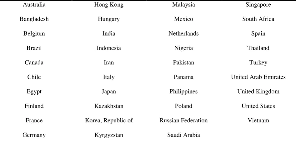
[image:14.595.76.550.462.696.2]Appendix A
Table A. Main trade partners of China in 2009 that are included into the study
Australia Hong Kong Malaysia Singapore
Bangladesh Hungary Mexico South Africa
Belgium India Netherlands Spain
Brazil Indonesia Nigeria Thailand
Canada Iran Pakistan Turkey
Chile Italy Panama United Arab Emirates
Egypt Japan Philippines United Kingdom
Finland Kazakhstan Poland United States
France Korea, Republic of Russian Federation Vietnam
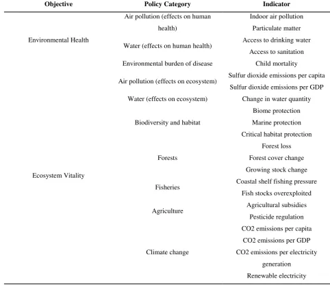
Appendix B
Table B. Indicators that Environmental Performance Index is comprised of
Objective Policy Category Indicator
Environmental Health
Air pollution (effects on human health)
Indoor air pollution Particulate matter
Water (effects on human health) Access to drinking water Access to sanitation Environmental burden of disease Child mortality
Ecosystem Vitality
Air pollution (effects on ecosystem) Sulfur dioxide emissions per capita Sulfur dioxide emissions per GDP Water (effects on ecosystem) Change in water quantity
Biodiversity and habitat
Biome protection Marine protection Critical habitat protection
Forests
Forest loss Forest cover change Growing stock change
Fisheries Coastal shelf fishing pressure Fish stocks overexploited
Agriculture Agricultural subsidies Pesticide regulation
Climate change
CO2 emissions per capita CO2 emissions per GDP CO2 emissions per electricity