Using Bilingual Comparable Corpora and Semi-supervised Clustering for
Topic Tracking
Fumiyo Fukumoto
Interdisciplinary Graduate School of Medicine and Engineering
Univ. of Yamanashi
Yoshimi Suzuki
Interdisciplinary Graduate School of Medicine and Engineering
Univ. of Yamanashi
Abstract
We address the problem dealing with
skewed data, and propose a method for estimating effective training stories for the topic tracking task. For a small number of labelled positive stories, we extract story pairs which consist of positive and its as-sociated stories from bilingual comparable corpora. To overcome the problem of a large number of labelled negative stories, we classify them into some clusters. This is done by using k-means with EM. The results on the TDT corpora show the ef-fectiveness of the method.
1 Introduction
With the exponential growth of information on the Internet, it is becoming increasingly difficult to find and organize relevant materials. Topic Track-ing defined by the TDT project is a research area to attack the problem. It starts from a few sample stories and finds all subsequent stories that discuss the target topic. Here, a topic in the TDT con-text is something that happens at a specific place and time associated with some specific actions. A wide range of statistical and ML techniques have been applied to topic tracking(Carbonell et. al, 1999; Oard, 1999; Franz, 2001; Larkey, 2004). The main task of these techniques is to tune the parameters or the threshold to produce optimal re-sults. However, parameter tuning is a tricky issue for tracking(Yang, 2000) because the number of initial positive training stories is very small (one to four), and topics are localized in space and time. For example, ‘Taipei Mayoral Elections’ and ‘U.S. Mid-term Elections’ are topics, but ‘Elections’ is not a topic. Therefore, the system needs to esti-mate whether or not the test stories are the same
topic with few information about the topic. More-over, the training data is skewed data, i.e. there is a large number of labelled negative stories com-pared to positive ones. The system thus needs to balance the amount of positive and negative train-ing stories not to hamper the accuracy of estima-tion.
In this paper, we propose a method for esti-mating efficient training stories for topic track-ing. For a small number of labelled positive sto-ries, we use bilingual comparable corpora (TDT1-3 English and Japanese newspapers, Mainichi and Yomiuri Shimbun). Our hypothesis using bilin-gual corpora is that many of the broadcasting sta-tion from one country report local events more fre-quently and in more detail than overseas’ broad-casting stations, even if it is a world-wide famous ones. Let us take a look at some topic from the TDT corpora. A topic, ‘Kobe Japan quake’ from the TDT1 is a world-wide famous one, and 89 stories are included in the TDT1. However, Mainichi and Yomiuri Japanese newspapers have much more stories from the same period of time, i.e. 5,029 and 4,883 stories for each. These obser-vations show that it is crucial to investigate the use of bilingual comparable corpora based on the NL techniques in terms of collecting more information about some specific topics. We extract Japanese stories which are relevant to the positive English stories using English-Japanese bilingual corpora, together with the EDR bilingual dictionary. The associated story is the result of alignment of a Japanese term association with an English term as-sociation.
For a large number of labelled negative sto-ries, we classify them into some clusters us-ing labelled positive stories. We used a semi-supervised clustering technique which combines
labeled and unlabeled stories during clustering. Our goal for semi-supervised clustering is to clas-sify negative stories into clusters where each clus-ter is meaningf ul in terms of class distribution provided by one cluster of positive training sto-ries. We introducek-means clustering that can be viewed as instances of the EM algorithm, and clas-sify negative stories into clusters. In general, the number of clusterskfor thek-means algorithm is not given beforehand. We thus use the Bayesian Information Criterion (BIC) as the splitting crite-rion, and select the proper number fork.
2 Related Work
Most of the work which addresses the small num-ber of positive training stories applies statistical techniques based on word distribution and ML techniques. Allan et. al explored on-line adaptive filtering approaches based on the threshold strat-egy to tackle the problem(Allan et. al, 1998). The basic idea behind their work is that stories closer together in the stream are more likely to discuss re-lated topics than stories further apart. The method is based on unsupervised learning techniques ex-cept for its incremental nature. When a tracking query is first created from theNttraining stories, it is also given a threshold. During the tracking phase, if a story S scores over that threshold, S
is regarded to be relevant and the query is regen-erated as if S were among the Nt training sto-ries. This method was tested using the TDT1 cor-pus and it was found that the adaptive approach is highly successful. But adding more than four training stories provided only little help, although in their approach, 12 training stories were added. The method proposed in this paper is similar to Allan’s method, however our method for collect-ing relevant stories is based on story pairs which are extracted from bilingual comparable corpora.
The methods for finding bilingual story pairs are well studied in the cross-language IR task, or MT systems/bilingual lexicons(Dagan, 1997). Much of the previous work uses cosine similar-ity between story term vectors with some weight-ing techniques(Allan et. al, 1998) such as TF-IDF, or cross-language similarities of terms. However, most of them rely on only two stories in question to estimate whether or not they are about the same topic. We use multiple-links among stories to produce optimal results.
In the TDT tracking task, classifying negative
stories into meaningf ul groups is also an im-portant issue to track topics, since a large num-ber of labelled negative stories are available in the TDT context. Basu et. al. proposed a method usingk-means clustering with the EM al-gorithm, where labeled data provides prior infor-mation about the conditional distribution of hid-den category labels(Basu, 2002). They reported that the method outperformed the standard random seeding and COP-k-means(Wagstaff, 2001). Our method shares the basic idea with Basu et. al. An important difference with their method is that our method does not require the number of clustersk
in advance, since it is determined during cluster-ing. We use the BIC as the splitting criterion, and estimate the proper number for k. It is an impor-tant feature because in the tracking task, no knowl-edge of the number of topics in the negative train-ing stories is available.
3 System Description
The system consists of four procedures: extracting bilingual story pairs, extracting monolingual story pairs, clustering negative stories, and tracking.
3.1 Extracting Bilingual Story Pairs
We extract story pairs which consist of positive English story and its associated Japanese stories using the TDT English and Mainichi and Yomi-uri Japanese corpora. To address the optimal pos-itive English and their associated Japanese stories, we combine the output of similarities(multiple-links). The idea comes from speech recognition where two outputs are combined to yield a better result in average. Fig.1 illustrates multiple-links. The TDT English corpus consists of training and test stories. Training stories are further divided into positive(black box) and negative stories(doted box). Arrows in Fig.1 refer to an edge with simi-larity value between stories. In Fig.1, for example, whether the storyJ2discusses the target topic, and is related toE1or not is determined by not only the value of similarity betweenE1andJ2, but also the similarities betweenJ2andJ4,E1andJ4.
Extracting story pairs is summarized as follows: Let initialpositivetraining storiesE1,· · ·,Embe initial node, and each Japanese storiesJ1,· · ·,Jm be node or terminal node in the graphG. We cal-culate cosine similarities betweenEi(1≤i≤m) andJj(1≤j≤m)1. In a similar way, we
training stories
test stories time lines TDT English corpus
E1 E2 E3
edge(E1,J1)
edge(E1,J4)
time lines
Mainichi and Yomiuri Japanese corpora topic
J1 J2 J3 J4 J5 J6 Jm’
edge(J2,J4)
[image:3.595.70.293.63.219.2]not topic
Figure 1: Multiple-links among stories
late similarities betweenJkandJl(1≤k,l≤m). If the value of similarity between nodes is larger than a certain threshold, we connect them by an edge(bold arrow in Fig.1). Next, we delete an edge which is not a constituent of maximal connected sub-graph(doted arrow in Fig.1). After eliminat-ing edges, we extract pairs of initial positive En-glish story Ei and Japanese story Jj as a linked story pair, and add associated Japanese story Jj to the training stories. In Fig.1, E1, J2, and J4
are extracted. The procedure for calculating co-sine similarities betweenEiandJjconsists of two sub-steps: extracting terms, and estimating bilin-gual term correspondences.
Extracting terms
The first step to calculate similarity between
Ei and Jj is to align a Japanese term with its associated English term using the bilingual dic-tionary, EDR. However, this naive method suf-fers from frequent failure due to incompleteness of the bilingual dictionary. Let us take a look at the Mainichi Japanese newspaper stories. The to-tal number of terms(words) from Oct. 1, 1998 to Dec. 31, 1998, was 528,726. Of these, 370,013 terms are not included in the EDR bilingual dic-tionary. For example, ’エンデバー(Endeavour)’ which is akeyterm for the topic ‘Shuttle Endeav-our mission for space station’ from the TDT3 cor-pus is not included in the EDR bilingual dictio-nary. New terms which fail to segment by dur-ing a morphological analysis are also a problem in calculating similarities between stories in mono-lingual data. For example, a proper noun ‘首都大 学東京’(Tokyo Metropolitan Univ.) is divided into three terms, ‘首都’ (Metropolitan), ‘大学(Univ.)’,
Japanese story pairs.
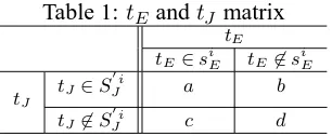
Table 1:tEandtJ matrix
tE
tE∈siE tE∈siE
tJ
tJ ∈S
i
J a b
tJ ∈S
i
J c d
and ‘東京(Tokyo)’. To tackle these problems, we conducted term extraction from a large collection of English and Japanese corpora. There are several techniques for term extraction(Chen, 1996). We usedn-gram model with Church-Gale smoothing, since Chen reported that it outperforms all existing methods on bigram models produced from large training data. The length of the extracted terms does not have a fixed range2. We thus applied the normalization strategy which is shown in Eq.(1) to each length of the terms to bring the probabil-ity value into the range[0,1]. We extracted terms whose probability value is greater than a certain threshold. Words from the TDT English(Japanese newspaper) corpora are identified if they match the extracted terms.
simnew =
simold−simmin
simmax−simmin
(1)
Bilingual term correspondences
The second step to calculate similarity between
Ei andJjis to estimate bilingual term correspon-dences usingχ2statistics. We estimated bilingual term correspondences with a large collection of English and Japanese data. More precisely, letEi be an English story (1 ≤ i≤n), where nis the number of stories in the collection, andSJi denote the set of Japanese stories with cosine similarities higher than a certain threshold valueθ: Si
J ={Jj
| cos(Ei, Jj) ≥ θ}. Then, we concatenate con-stituent Japanese stories ofSJi into one storySJi, and construct a pseudo-parallel corpusP P CEJ of English and Japanese stories: P P CEJ = { {Ei,
SJi} |SJi =0}. Suppose that there are two crite-ria, monolingual termtEin English story andtJin Japanese story. We can determine whether or not a particular term belongs to a particular story. Con-sequently, terms are divided into four classes, as shown in Table 1. Based on the contingency table of co-occurence frequencies oftEandtJ, we esti-mate bilingual term correspondences according to the statistical measureχ2.
χ2(tE, tJ) =
(ad−bc)2
(a+b)(a+c)(b+d)(c+d) (2)
[image:3.595.341.494.71.134.2]We extract termtJ as a pair oftE which satisfies maximum value of χ2, i.e. maxtJ∈TJ χ2(tE,tJ),
whereTJ={tJ |χ2(tE,tJ)}. For the extracted En-glish and Japanese term pairs, we conducted semi-automatic acquisition, i.e. we manually selected bilingual term pairs, since our source data is not a clean parallel corpus, but an artificially gener-ated noisy pseudo-parallel corpus, it is difficult to compile bilingual terms full-automatically(Dagan, 1997). Finally, we align a Japanese term with its associated English term using the selected bilin-gual term correspondences, and again calculate cosine similarities between Japanese and English stories.
3.2 Extracting Monolingual Story Pairs
We noted above that our source data is not a clean parallel corpus. Thus the difference of dates be-tween bilingual stories is one of the key factors to improve the performance of extracting story pairs, i.e. stories closer together in the timeline are more likely to discuss related subjects. We therefore ap-plied a method for extracting bilingual story pairs from stories closer in the timelines. However, this often hampers our basic motivation for using bilin-gual corpora: bilinbilin-gual corpora helps to collect more information about the target topic. We there-fore extracted monolingual(Japanese) story pairs and added them to the training stories. Extract-ing Japanese monolExtract-ingual story pairs is quite sim-ple: LetJj(1≤j≤m) be the extracted Japanese story in the procedure, extracting bilingual story pairs. We calculate cosine similarities betweenJj andJk(1≤k≤n). If the value of similarity be-tween them is larger than a certain threshold, we addJkto the training stories.
3.3 Clustering Negative Stories
Our method for classifying negative stories into some clusters is based on Basu et. al.’s method(Basu, 2002) which usesk-means with the EM algorithm. K-means is a clustering algo-rithm based on iterative relocation that partitions a dataset into the number of k clusters, locally minimizing the average squared distance between the data points and the cluster centers(centroids). Suppose we classify X = { x1, · · ·, xN}, xi ∈
Rdinto kclusters: one is the cluster which con-sists of positive stories, and other k-1 clusters consist of negative stories. Here, which clusters does each negative story belong to? The EM is
a method of finding the maximum-likelihood es-timate(MLE) of the parameters of an underlying distribution from a set of observed data that has missing value. K-means is essentially an EM on a mixture of k Gaussians under certain assump-tions. In the standardk-means without any initial supervision, the k-means are chosen randomly in the initial M-step and the stories are assigned to the nearest means in the subsequent E-step. For positive training stories, the initial labels are kept unchanged throughout the algorithm, whereas the conditional distribution for the negative stories are re-estimated at every E-step. We select the num-ber ofkinitial stories: one is the cluster center of positive stories, and otherk-1 stories are negative stories which have the topk-1 smallest value be-tween the negative story and the cluster center of positive stories. In Basu et. al’s method, the num-ber ofkis given by a user. However, for negative training stories, the number of clusters is not given beforehand. We thus developed an algorithm for estimatingk. It goes into action after each run of
k means3, making decisions about which sets of clusters should be chosen in order to better fit the data. The splitting decision is done by comput-ing the Bayesian Information Criterion which is shown in Eq.(3).
BIC(k=l) = llˆl(X)−
pl
2 ·logN (3)
wherellˆl(X)is the log-likelihood ofXaccording to the number ofk isl, N is the total number of training stories, and pl is the number of parame-ters ink=l. We setplto the sum ofkclass prob-abilities,km=1llˆ(Xm) , the number ofn·k cen-troid coordinates, and the MLE for the variance,
ˆ
ρ2. Here,nis the number of dimensions. ρˆ2, un-der the identical spherical Gaussian assumption, is:
ˆ
ρ2 = 1 N−k
i
(xi−μi)2 (4)
whereμi denotesi-th partition center. The proba-bilities are:
ˆ P(xi) =
Ri
N · 1
√
2πρˆnexp(−
1
2ˆρ2 ||xi−μi||
2)(5)
Ri is the number of stories that have μi as their closest centroid. The log-likelihood of ll(X)
3We set the maximum number ofkto 100 in the
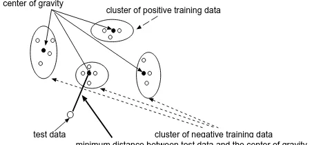
cluster of positive training data
cluster of negative training data test data
center of gravity
[image:5.595.67.293.66.171.2]minimum distance between test data and the center of gravity
Figure 2: Each cluster and a test story
is logiP(xi). It is taken at the maximum-likelihood point(story), and thus, focusing just on the setXm⊆Xwhich belongs to the centroidm and plugging in the MLE yields:
ˆ
ll(Xm) =−
Rm
2 log(2π)− Rm·n
2 log( ˆρ2)− Rm−k
2
+RmlogRm−RmlogN (1≤m≤k) (6)
We choose the number of kwhose value ofBIC
is highest.
3.4 Tracking
Each story is represented as a vector of terms with tf· idf weights in an n dimensional space, wherenis the number of terms in the collection. Whether or not each test story is positive is judged using the distance (measured by cosine similarity) between a vector representation of the test story and each centroid g of the clusters. Fig.2 illus-trates each cluster and a test story in the tracking procedure. Fig.2 shows that negative training sto-ries are classified into three groups. The centroid
gfor each cluster is calculated as follows:
g = (g1,· · ·, gn) = (
1 p
p
i=1
xi1,· · ·,1p
p
i=1
xin)(7)
wherexij(1≤j≤n) is thetf·idf weighted value of term jin the storyxi. The test story is judged by using these centroids. If the value of cosine similarity between the test story and the centroid with positive stories is smallest among others, the test story is declared to be positive. In Fig.2, the test story is regarded as negative, since the value between them is smallest. This procedure, is re-peated until the last test story is judged.
4 Experiments
4.1 Creating Japanese Corpus
We chose the TDT3 English corpora as our gold standard corpora. TDT3 consists of 34,600 sto-ries with 60 manually identified topics. We then
created Japanese corpora (Mainichi and Yomiuri newspapers) to evaluate the method. We annotated the total number of 66,420 stories from Oct.1, to Dec.31, 1998, against the 60 topics. Each story was labelled according to whether the story dis-cussed the topic or not. Not all the topics were present in the Japanese corpora. We therefore col-lected 1 topic from the TDT1 and 2 topics from the TDT2, each of which occurred in Japan, and added them in the experiment. TDT1 is collected from the same period of dates as the TDT3, and the first story of ‘Kobe Japan Quake’ topic starts from Jan. 16th. We annotated 174,384 stories of Japanese corpora from the same period for the topic. Ta-ble 2 shows 24 topics which are included in the Japanese corpora. ‘TDT’ refers to the evaluation data, TDT1, 2, or 3. ‘ID’ denotes topic number de-fined by the TDT. ‘OnT.’(On-Topic) refers to the number of stories discussing the topic. Bold font stands for the topic which happened in Japan. The evaluation of annotation is made by three humans. The classification is determined to be correct if the majority of three human judges agree.
4.2 Experiments Set Up
The English data we used for extracting terms is Reuters’96 corpus(806,791 stories) including TDT1 and TDT3 corpora. The Japanese data was 1,874,947 stories from 14 years(from 1991 to 2004) Mainichi newspapers(1,499,936 stories), and 3 years(1994, 1995, and 1998) Yomiuri newspapers(375,011 stories). All Japanese sto-ries were tagged by the morphological analysis Chasen(Matsumoto, 1997). English stories were tagged by a part-of-speech tagger(Schmid, 1995), and stop word removal. We appliedn-gram model with Church-Gale smoothing to noun words, and selected terms whose probabilities are higher than a certain threshold4. As a result, we obtained 338,554 Japanese and 130,397 English terms. We used the EDR bilingual dictionary, and translated Japanese terms into English. Some of the words had no translation. For these, we estimated term correspondences. Each story is represented as a vector of terms with tf·idf weights. We calcu-lated story similarities and extracted story pairs between positive and its associated stories5. In
4The threshold value for both English and Japanese was
0.800. It was empirically determined.
5The threshold value for bilingual story pair was 0.65, and
Table 2: Topic Name
TDT ID Topic name OnT. TDT ID Topic name OnT.
1 15 Kobe Japan quake 9,912
2 31015 Japan Apology to Korea 28 2 31023 Kyoto Energy Protocol 40 3 30001 Cambodian government coalition 48 3 30003 Pinochet trial 165 3 30006 NBA labor disputes 44 3 30014 Nigerian gas line fire 6 3 30017 North Korean food shortages 23 3 30018 Tony Blair visits China in Oct. 7 3 30022 Chinese dissidents sentenced 21 3 30030 Taipei Mayoral elections 353 3 30031 Shuttle Endeavour mission for space station 17 3 30033 Euro Introduced 152 3 30034 Indonesia-East Timor conflict 34 3 30038 Olympic bribery scandal 35 3 30041 Jiang’s Historic Visit to Japan 111 3 30042 PanAm lockerbie bombing trial 13 3 30047 Space station module Zarya launched 30 3 30048 IMF bailout of Brazil 28 3 30049 North Korean nuclear facility? 111 3 30050 U.S. Mid-term elections 123 3 30053 Clinton’s Gaza trip 74 3 30055 D’Alema’s new Italian government 37 3 30057 India train derailment 12
the tracking, we used the extracted terms together with all verbs, adjectives, and numbers, and repre-sented each story as a vector of these withtf·idf
weights.
We set the evaluation measures used in the TDT benchmark evaluations. ‘Miss’ denotes Miss rate, which is the ratio of the stories that were judged as YES but were not evaluated as such for the run in question. ‘F/A’ shows false alarm rate, which is the ratio of the stories judged as NO but were eval-uated as YES. The DET curve plots misses and false alarms, and better performance is indicated by curves more to the lower left of the graph. The detection cost function(CDet) is defined by Eq.(8).
CDet = (CM iss∗PM iss∗PT arget+
CF a∗PF a∗(1−PT arget))
PM iss = #M isses/#T argets
PF a = #F alseAlarms/#N onT argets (8)
CM iss,CF a, andPT argetare the costs of a missed
detection, false alarm, and priori probability of finding a target, respectively. CM iss, CF a, and
PT argetare usually set to 10, 1, and 0.02,
respec-tively. The normalized cost function is defined by Eq.(9), and lower cost scores indicate better per-formance.
(CDet)N orm = CDet/M IN(CM iss∗PT arget, CF a
∗(1−PT arget)) (9)
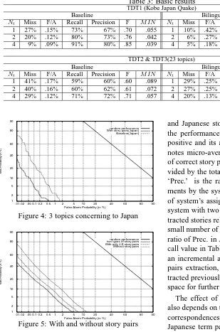
4.3 Basic Results
Table 3 summaries the tracking results. M IN
denotes M IN(CDet)N orm which is the value of
(CDet)N orm at the best possible threshold. Nt
is the number of initial positive training stories. We recall that we used subset of the topics de-fined by the TDT. We thus implemented Allan’s method(Allan et. al, 1998) which is similar to our method, and compared the results. It is based
1 2 5 10 20 40 60 80 90
.01 .02 .05 0.1 0.2 0.5 1 2 5 10 20 40 60 80 90
Miss Probability (in %)
False Alarm Probability (in %)
random performance With story pairs Baseline
Figure 3: Tracking result(23 topics)
on a tracking query which is created from the top 10 most commonly occurring features in the Nt stories, with weight equal to the number of times the term occurred in those stories multiplied by its incremental idf value. They used a shallow tag-ger and selected all nouns, verbs, adjectives, and numbers. We added the extracted terms to these part-of-speech words to make their results compa-rable with the results by our method. ‘Baseline’ in Table 3 shows the best result with their method among varying threshold values of similarity be-tween queries and test stories. We can see that the performance of our method was competitive to the baseline at everyNtvalue.
Fig.3 shows DET curves by both our method and Allan’s method(baseline) for 23 topics from the TDT2 and 3. Fig.4 illustrates the results for 3 topics from TDT2 and 3 which occurred in Japan. To make some comparison possible, only theNt= 4 is given for each. Both Figs. show that we have an advantage using bilingual comparable corpora.
4.4 The Effect of Story Pairs
[image:6.595.92.506.76.203.2]Table 3: Basic results TDT1 (Kobe Japan Quake)
Baseline Bilingual corpora & clustering
Nt Miss F/A Recall Precision F M IN Nt Miss F/A Recall Precision F M IN
1 27% .15% 73% 67% .70 .055 1 10% .42% 90% 74% .81 .023
2 20% .12% 80% 73% .76 .042 2 6% .27% 93% 76% .83 .013
4 9% .09% 91% 80% .85 .039 4 5% .18% 96% 81% .88 .012
TDT2 & TDT3(23 topics)
Baseline Bilingual corpora & clustering
Nt Miss F/A Recall Precision F M IN Nt Miss F/A Recall Precision F M IN
1 41% .17% 59% 60% .60 .089 1 29% .25% 71% 54% .61 .059
2 40% .16% 60% 62% .61 .072 2 27% .25% 73% 55% .63 .054
4 29% .12% 71% 72% .71 .057 4 20% .13% 80% 73% .76 .041
1 2 5 10 20 40 60 80 90
.01 .02 .05 0.1 0.2 0.5 1 2 5 10 20 40 60 80 90
Miss Probability (in %)
False Alarm Probability (in %)
random performance With story pairs(Japan) Baseline(Japan)
Figure 4: 3 topics concerning to Japan
1 2 5 10 20 40 60 80 90
.01 .02 .05 0.1 0.2 0.5 1 2 5 10 20 40 60 80 90
Miss Probability (in %)
False Alarm Probability (in %)
random performance two types of story pairs With only J-E story pairs Without story pairs
Figure 5: With and without story pairs
Japanese stories in question, and without story pairs, and (ii) the results of story pairs by vary-ing values ofNt. Fig.5 illustrates DET curves for 23 topics,Nt=4.
As can be clearly seen from Fig.5, the re-sult with story pairs improves the overall perfor-mance, especially the result with two types of story pairs was better than that with only English
Table 4: Performance of story pairs(24 topics) Two types of story pairs J-E story pairs
Nt Rec. Prec. F Rec. Prec. F
1 30% 82% .439 28% 80% .415
2 36% 85% .506 33% 82% .471
4 45% 88% .595 42% 79% .548
and Japanese stories in question. Table 4 shows the performance of story pairs which consist of positive and its associated story. Each result de-notes micro-averaged scores. ‘Rec.’ is the ratio of correct story pair assignments by the system di-vided by the total number of correct assignments. ‘Prec.’ is the ratio of correct story pair assign-ments by the system divided by the total number of system’s assignments. Table 4 shows that the system with two types of story pairs correctly ex-tracted stories related to the target topic even for a small number of positive training stories, since the ratio of Prec. inNt= 1 is 0.82. However, each re-call value in Table 4 is low. One solution is to use an incremental approach, i.e. by repeating story pairs extraction, new story pairs that are not ex-tracted previously may be exex-tracted. This is a rich space for further exploration.
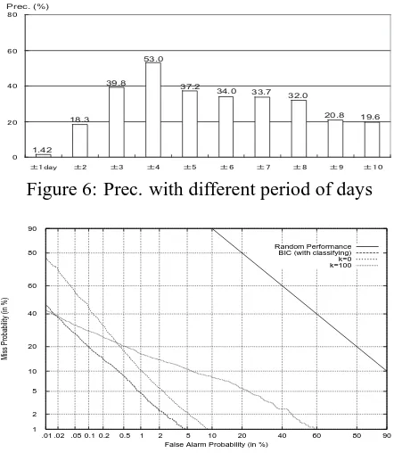
The effect of story pairs for the tracking task also depends on the performance of bilingual term correspondences. We obtained 1,823 English and Japanese term pairs in all when a period of days was ±4. Fig.6 illustrates the result using differ-ent period of days(±1 to±10). For example, ‘±1’ shows that the difference of dates between English and Japanese story pairs is less than ±1. Y-axis shows the precision which is the ratio of correct term pairs by the system divided by the total num-ber of system’s assignments. Fig.6 shows that the difference of dates between bilingual story pairs, affects the overall performance.
4.5 The Effect ofk-means with EM
㪇 㪉㪇 㪋㪇 㪍㪇 㪏㪇
㫧㪈㪻㪸㫐 㫧㪉 㫧㪊 㫧㪋 㫧㪌 㫧㪍 㫧㪎 㫧㪏 㫧㪐 㫧㪈㪇
Prec. (%)
1.42 18.3
39.8 53.0
37.2 34.0
33.7 32.0
[image:8.595.70.291.62.316.2]20.8 19.6
Figure 6: Prec. with different period of days
1 2 5 10 20 40 60 80 90
.01 .02 .05 0.1 0.2 0.5 1 2 5 10 20 40 60 80 90
Miss Probability (in %)
False Alarm Probability (in %)
Random Performance BIC (with classifying) k=0 k=100
Figure 7: BIC v.s. fixedkfork-means with EM
positive by calculating cosine similarities between the test story and each centroid of negative and positive stories. Further, to examine the effect of using the BIC, we compared with choosing a pre-definedk, i.e. k=10, 50, and 100. Fig.7 illustrates part of the result fork=100. We can see that the method without classifying negative stories(k=0) does not perform as well and results in a high miss rate. This result is not surprising, because the size of negative training stories is large compared with that of positive ones, and therefore, the test story is erroneously judged as NO. Furthermore, the result indicates that we need to run BIC, as the result was better than the results with choosing any number of pre-definedk, i.e. k=10, 50, and 100. We also found that there was no correlation between the number of negative training stories for each of the 24 topics and the number of clusterskobtained by the BIC. The minimum number of clusters kwas 44, and the maximum was 100.
5 Conclusion
In this paper, we addressed the issue of the differ-ence in sizes between positive and negative train-ing stories for the tracktrain-ing task, and investigated the use of bilingual comparable corpora and semi-supervised clustering. The empirical results were encouraging. Future work includes (i) extend-ing the method to an incremental approach for extracting story pairs, (ii) comparing our cluster-ing method with the other existcluster-ing methods such
asX-means(Pelleg, 2000), and (iii) applying the method to the TDT4 for quantitative evaluation.
Acknowledgments
This work was supported by the Grant-in-aid for the JSPS, Support Center for Advanced Telecom-munications Technology Research, and Interna-tional Communications Foundation.
References
J.Allan and R.Papka and V.Lavrenko, On-line new event
detection and tracking, Proc. of the DARPA Workshop,
1998.
J.Allan and V.Lavrenko and R.Nallapti, UMass at TDT 2002, Proc. of TDT Workshop, 2002.
S.Basu and A.Banerjee and R.Mooney, Semi-supervised clustering by seeding, Proc. of ICML’02, 2002.
J.Carbonell et. al, CMU report on TDT-2: segmentation, detection and tracking, Proc. of the DARPA Workshop,
1999.
S.F.Chen and J.Goodman, An empirical study of smoothing
techniques for language modeling, Proc. of the ACL’96,
pp. 310-318, 1996.
N.Collier and H.Hirakawa and A.Kumano, Machine
trans-lation vs. dictionary term transtrans-lation - a comparison for English-Japanese news article alignment, Proc. of
COL-ING’02, pp. 263-267, 2002.
I.Dagan and K.Church, Termight: Coordinating humans and
machines in bilingual terminology acquisition, Journal of
MT, Vol. 20, No. 1, pp. 89-107, 1997.
M.Franz and J.S.McCarley, Unsupervised and supervised clustering for topic tracking, Proc. of SIGIR’01, pp.
310-317, 2001.
L.S.Larkey et. al, Language-specific model in multilingual
topic tracking, Proc. of SIGIR’04, pp. 402-409, 2004.
Y.Matsumoto et. al, Japanese morphological analysis system
chasen manual, NAIST Technical Report, 1997.
D.W.Oard, Topic tracking with the PRISE information
re-trieval system, Proc. of the DARPA Workshop, pp.
94-101, 1999.
D.Pelleg and A.Moore, X-means: Extending K-means with
efficient estimation of the number of clusters, Proc. of ICML’00, pp. 727-734, 2000.
H.Schmid, Improvements in part-of-speech tagging with an
application to german, Proc. of the EACL SIGDAT Work-shop, 1995.
K.Wagstaff et. al, Constrained K-means clustering with background knowledge, Proc. of ICML’01, pp. 577-584,
2001.