Munich Personal RePEc Archive
Exchange Rate Undervaluation and
Sectoral Performance of the South
African Economy
Njindan Iyke, Bernard
University of South Africa
1 March 2016
1
Exchange Rate Undervaluation and Sectoral Performance of the South African Economy
Bernard Njindan Iyke1
Department of Economics University of South Africa
P. O. Box 392, UNISA 0003, Pretoria
South Africa
Email: benitoflex@gmail.com/niykeb@unisa.ac.za
Previous Version: October 2014
This Version: March 2016
1
2
Exchange Rate Undervaluation and Sectoral Performance of the South African Economy
Abstract
The paper uncovers the channels through which real exchange rate undervaluation influences the performance of the South African economy. We decompose the South African economy into three sectors, namely: agriculture, industry, and service. Using the OLS (with Newey-West and robust standard errors), and GMM estimation techniques; an annual time series data covering the period 1962-2014; and a standard regression model for each sector, we find: (i) real exchange rate undervaluation to exert positive impact on economic performance by enhancing agricultural sector, and industrial sector performance; (ii) real exchange rate undervaluation to exert a negative impact on economic performance by reducing the performance of the service sector.
JEL Classification:C10, F21, F31
Keywords: Exchange Rate Undervaluation, Sectoral Performance, South Africa
1. Introduction
The exchange rate has remained one of the most widely discussed macroeconomic variables
throughout the world. The main concern is clear, as most theoretical and empirical studies show
– a poorly managed exchange rate could prove disastrous for the growth prospects of an
economy. To this end, some cross-country studies have emphasized the need to avoid overvalued
currencies (see, for instance, Razin and Collins 1997; Johnson et al. 2007; Rajan and
Subramanian 2007). The main argument advanced by these studies is that an overvalued
3
current account deficits, balance-of-payment crises, corruption, rent-seeking activities, among
others (see Fischer 1993; Rodrik 2008).
Overvaluation is the aspect of exchange rate misalignment that has been found undesirable for
economic growth in most empirical studies. Real misalignment of exchange rates in the form of
undervaluation (albeit moderate undervaluation), however, has been found to be desirable for
economic growth. Indeed, some empirical studies have found undervaluation to stimulate growth
(see Bhalla 2007; Gala 2008; Gluzmann et al. 2007; Rodrik 2008). There is even empirical
evidence which shows that most Eastern Asian countries, notably, Japan, South Korea, Taiwan,
Hong Kong, Singapore, and China have used undervalued currencies to their advantage (see
Dollar 1992).
While the growth-effect of real exchange rate undervaluation has been well-established in the
literature, the channel through which this occurs is actively being explored (see Wang and Barret
2007; Rodrik 2008). Our objective, in this paper, is to account for the channels through which
real exchange rate undervaluation affects the performance of the South African economy. This is
important because exchange rate policies aimed at stimulating sectoral performance will be
better implemented if the policymaker has a clear knowledge of how each sector reacts to such
policies. More so, the South African rand has depreciated rapidly in recent years. Hence, this
paper serves to uncover the sectors which responded favourably (unfavourably) to this
depreciation. We consider three main sectors of the South African economy, namely: agriculture,
industry, and services. Then, we estimate the impact of real exchange rate undervaluation on
each of these sectors. To the best of our knowledge, this paper is the first to explore the impact of
real exchange rate undervaluation on the performance of the South African economy.
Following standard approaches in the literature, we fit a standard regression model for each
sector. To estimate these regression models, we use the Ordinary Least Squares (OLS), and the
Generalized Method of Moments (GMM) estimators. We define real exchange rate
undervaluation in a fashion similar to Rodrik (2008), so that a positive coefficient of this term
implies overvaluation mars sectoral performance, and vice versa. Our measure of real exchange
4
a quantile regression estimator whereas Rodrik (2008) uses the within-effects estimator. We also
construct an alternative measure of real exchange rate undervaluation by extracting the cyclical
component of the real exchange rate index to analyze the sensitivity of the results to our measure
of undervaluation. This new measure is constructed using the Hodrick-Prescott filter. Our
interpretation of this alternative measure of real exchange rate undervaluation is the same as the
first. This is another direction in which our paper varies from previous studies.
We establish two important results in this paper. First, real exchange rate undervaluation exerts
positive impact on the performance of the South African economy by enhancing agricultural, and
industrial sector performance. Second, real exchange rate undervaluation exerts a negative
impact on the performance of the South African economy by reducing the performance of the
service sector. We emphasize, here, that our results remain robust to serial correlation of the
errors, heteroskedasticity of the variance, endogeneity, variable omission, and the measure of
real exchange undervaluation used in this paper.
In the next section, we present our methodology and the data. In Section 3, we present and
discuss our results. We provide our concluding remarks in the last section.
2. Methodology
2.1 Baseline Regression
The core objective of this paper is to investigate the channels through which real exchange rate
undervaluation affects the performance of the South African economy. Defining a standard
measure of real exchange rate undervaluation is, therefore, central to achieving this objective.
Different measures could be found in the exchange rate literature. In this paper, however, we
construct a measure of real exchange rate undervaluation which is very similar in meaning and
procedure as the one presented in Rodrik (2008). Essentially, we construct this index by
5
(𝑃𝑡) and the U.S. (𝑃𝑡∗) from the World Bank’s World Development Indicators (WDI) database.2
Once we extract these variables, we set up the following equation:
𝑙𝑙𝑅𝑅𝑅𝑡 = ln �𝑒𝑡𝑃𝑡 ∗
𝑃𝑡�, (1)
where 𝑡 is the time window and 𝑙𝑙𝑅𝑅𝑅𝑡 is the natural logarithm of real exchange rate. By
interpretation, when RER is increasing, it implies that the Rand is depreciating relative to the
dollar in real terms. Eichengreen and Gupta (2013) have also utilized this measure in their paper.
Nontraded goods are known to be cheaper in developing countries than in developed countries.
This is the main implication of the Balassa-Samuelson-Bhagwati effect (see Balassa, 1964;
Samuelson, 1964; and Bhagwati, 1984). For this reason, Rodrik (2008), Gala (2008), and
Gluzmann et al. (2012) propose that we account for the Balassa-Samuelson-Bhagwati effect in
the final measure of real exchange rate undervaluation. Hence, we proceed to fit a model which
accounts for the Balassa-Samuelson-Bhagwati effect in the following fashion:
𝑙𝑙𝑅𝑅𝑅𝑡 =𝜂+𝜙𝑙𝑙𝐺𝐺𝑃𝑡+𝜀𝑡, (2)
where 𝜂 and 𝜙 are parameters of the model, 𝐺𝐺𝑃𝑡 is real per capita GDP of South Africa
divided by real per capita GDP of the U.S. at time period 𝑡, 𝑙𝑙 is the natural logarithm, and 𝜀𝑡 is
the error term at time 𝑡.3 The a priori assumption made on 𝜙 is that it is negative and significant.
In practice, various studies have found 𝜙 to be negative and significant (see Gala, 2008; Rodrik,
2008; Gluzmann et al., 2012; Vieira and MacDonald, 2012, for example). The main departure of
our study from other studies, in the construction of this index, is the estimation technique
employed to estimate (2). Gala (2008), Rodrik (2008), and Gluzmann et al. (2012), for instance,
estimate (2) using the within-effects technique. In our case, we estimate (2) using the quantile
regression technique. Our main motivation for using the quantile regression technique is to
moderate the impact of outliers on the final value of 𝜙. As a final step for constructing the real
2
We compared this index to the one based on relative GDP deflators of the U.S. and South Africa but there is no significant statistical gain. Data on this other measure of real exchange rate undervaluation is available upon request. 3
6
exchange rate undervaluation index, we find the difference between the actual real exchange in
(1) and the adjusted Balassa-Samuelson-Bhagwati rate as:
𝑙𝑙𝑄𝑅𝑅𝑅𝑡 =𝑙𝑙𝑅𝑅𝑅𝑡− 𝑙𝑙𝑅𝑅𝑅�𝑡, (3)
where 𝑙𝑙𝑅𝑅𝑅�𝑡 denotes the predicted values of the natural logarithm of the real exchange rate in
(2); and 𝑙𝑙𝑄𝑅𝑅𝑅𝑡 is the real exchange rate undervaluation index.
The alternative measure of real exchange undervaluation we use is based on filtering techniques.
We decompose the real exchange rate index in (1) into trend and cyclical components and use
the cyclical component as the measure of real exchange rate undervaluation. To provide a
theoretically defensible cyclical component of the real exchange rate, we employ the most used
filter in empirical macroeconomics, the Hodrick-Prescott (HP) filter proposed by Hodrick and
Prescott (1997).4 The cyclical component of the real exchange rate, which we derive from the HP
filter, is named HPRER.
Having constructed the measure of real exchange rate undervaluation; we fit a standard
regression model for each of the sectors. To conserve space, we only show the relationship
between our main measure of real exchange rate undervaluation and the three sectors of the
South African economy as follows:
𝑆𝑅𝑆𝑖𝑡 =𝜏0+𝜏1𝑙𝑙𝑄𝑅𝑅𝑅𝑡+Ω𝑆𝐶𝐶𝐶𝑖𝑡+ω𝑖𝑡, (4)
where 𝑆𝑅𝑆𝑖𝑡 is sector 𝑖’s contribution to GDP at time t. 𝜏 and Ω are the parameters of the model;
𝜔𝑖𝑡 is the error term for sector 𝑖 at time 𝑡. 𝑆𝐶𝐶𝐶𝑖𝑡 is a vector of 1xq control variables denoting the factors that determine sectoral performance, apart from real exchange rate undervaluation.
For simplicity, we assume that all sectors are influence by the same kind of factors. This
assumption is necessary to keep our estimates tractable. Ω is a vector of qx1 parameters to be
estimated. Our objective parameter is 𝜏1, the parametric measure of the impact of changes in real
4
7
exchange rate undervaluation on sectoral performance. Notice that (4) resembles the standard
neoclassical regressions used in various empirical studies. The clear variation is the absence of
the initial level of sectoral performance term. As control variables, we include physical capital,
human capital, population growth, inflation rate, real interest rate, terms of trade, trade openness,
and the size of credit from the banking sector to private sector.
2.2 Testing for Stationarity
In this paper, we examine the stationary status of the variables employed. The reason for
examining the stationary properties of these variables is a stylized fact. Time series variables are
known to exhibit non-mean reverting features. Such features, if uncontrolled for, result in
estimates that are spurious. The standard tests for stationarity that we use are the Phillips-Perron
(PP) test due to Phillips and Perron (1988), and the Dickey-Fuller Generalized Least Squares
(DF-GLS) test due to Elliot et al. (1996).5 These two tests are chosen because they are able to
control for serial correlation when testing for unit roots.
2.3 Data and Estimation Techniques
Our data on the variables used in this paper are obtained from three sources.6 The dataset is
annual and covers the period 1962-2014. The data on human capital (HC)7, and terms of trade
(TOT) are taken from the Penn World Tables, version 7.1 compiled by Heston et al. (2012). TOT
is calculated as the price of export divided by the price of import.8 The data on private credit by
deposit money banks and other financial institutions as a percentage of GDP (PRIVY) comes
from the World Bank’s Global Financial Development. The remaining variables, namely:
physical capital (K) measured as gross capital formation as a percentage of GDP), population
growth (POP), inflation rate (INF), trade openness (OPEN), and real interest rate (RIR) are
extracted from the World Development Indicators (WDI, 2015). We define the performance of
the sectors as: (i) agriculture, value added (% of GDP); (ii) industry, value added (% of GDP);
and (iii) service value added (% of GDP). These variables are extracted from WDI (2015).
5
These are well-known stationarity tests, so we save space by not describing them here. The interested reader is referred to the references cited herein.
6
The complete dataset is available upon request. 7
Observations on HC are not available beyond 2010 in the sourced database. We updated it using the Barro-Lee database (see Barro and Lee, 2013) and interpolation.
8
8
We estimate (4) using the OLS estimator (with Newey-West and robust standard errors9), and
the generalized method of moments (GMM) estimator. By using the Newey-West errors and the
robust standard errors, we are able to report coefficient estimates which are robust to potential
autocorrelation and heteroskedasticity in our dataset. We employ instrumental variables using the
GMM estimator to cater for potential endogeneity problem in (4) which might bias the
coefficient estimates.
3. Results
3.1 Results for Stationarity Tests
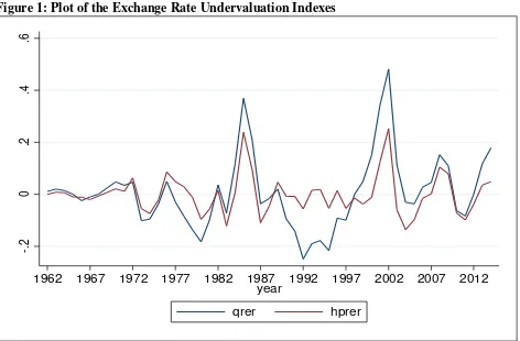
We begin our analysis by first constructing the real exchange undervaluation indexes discussed
earlier, and examining their stationary properties.10 Figure 1 in Appendix A shows how the two
indexes compare to each other. The two indexes appear fairly close in resemblance.11 Thus, the
sensitivity analysis that we perform later is appropriate. In addition, we analyze the stationary
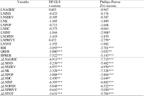
properties of the other variables utilized in this paper. Table 1 shows the results of the
stationarity tests of the variables. With the exception of the real interest rate and the two
measures of exchange rate undervaluation, all the other variables are non-stationary at the
conventional levels of significance.
To ensure that the non-stationary variables become stationary, we differenced them once. Table
1 also shows the results of the stationarity tests of the variables in their first differences. As the
results indicate, these variables are now stationary at the conventional levels. Testing for
cointegrating relationships may not be necessary since the variables have mixed order of
integration.
9
See Newey and West (1987), for these errors. 10
We used 1000 bootstrap replications for the quantile regression based undervaluation index. The estimated regression was 𝑙𝑙𝑅𝑅𝑅𝑡= .794−.627𝑙𝑙𝐺𝐺𝑃𝑡; t-statistic and p-value for the 𝑙𝑙𝐺𝐺𝑃𝑡 coefficient were -8.79 and 0.00, respectively. This indicates a strong evidence of the Balassa-Samuelson-Bhagwati effect. We set the smoothing parameter to 6.25, for the HP based undervaluation index.
11
9
Table 1: Tests for Stationarity of the Variables in Levels and First Difference
Variable DF-GLS
t-statistic Phillips-Perron Z(t)-statistic LNAGRIC LNIND LNSERV LNK LNPOP LNHC LNINF LNOPEN LNPRIVY LNTOT RIR QRER HPRER 0.603 -0.423 -0.305 -1.485 -0.713 -0.375 -1.044 -1.419 0.472 -1.555 -3.055*** -3.880*** -7.522*** -0.967 -0.176 -0.387 -1.889 -1.668 -0.063 -2.908* -1.870 -2.759* -1.982 -3.701*** -3.052** -5.143*** ∆LNAGRIC ∆LNIND ∆LNSERV ∆LNK ∆LNPOP ∆LNHC ∆LNINF ∆LNOPEN ∆LNPRIVY ∆LNTOT -6.913*** -5.239*** -4.957*** -3.328*** -3.888*** -2.450** -6.395*** -5.048*** -9.642*** -3.631*** -7.715*** -5.482*** -4.950*** -7.328*** -3.804*** -2.649* -6.882*** -6.522*** -5.050*** -5.704*** Notes:
(1) The optimal lag for DF-GLS is chosen by Minimum MAIC; the optimal lag for Phillips-Perron is based on Newey-West.
(2) LN is the natural logarithm operator. (3) ∆ is the first difference operator.
(4) *, **, *** indicate rejection of the null hypothesis at 10%, 5%, and 1%, respectively.
3.2 Real Exchange Rate Undervaluation and Sectoral Performance
We have no reason to worry about spurious outcomes, since all the variables are free from unit
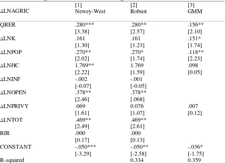
roots. Next, we present the results of the regression estimates for the agricultural sector. These
results are shown in Table 2a. Panels [1] and [2] show the OLS estimates using the Newey-West
errors and the robust standard errors, respectively. For this estimation technique, exchange rate
undervaluation positively and significantly affects agricultural sector performance. Panel [3]
reports the results obtained when we corrected for potential endogeneity using the GMM
technique. For this case as well, the exchange rate undervaluation affects agricultural sector
performance positively and significantly. The GMM estimate of the real exchange rate
10
presence of endogeneity problems in the OLS estimates may have led to the slightly
overestimated impact of the real exchange rate undervaluation on agricultural sector
performance. It is fair, nevertheless, to say that exchange rate affects agricultural sector
[image:11.612.72.531.187.519.2]performance positively, if anything at all.
Table 2a: Exchange Rate Undervaluation and Agriculture Sector Performance
∆LNAGRIC [1] Newey-West [2] Robust [3] GMM QRER ∆LNK ∆LNPOP ∆LNHC ∆LNINF ∆LNOPEN ∆LNPRIVY ∆LNTOT RIR CONSTANT R-squared .280*** [3.38] .161 [1.30] .270** [2.02] 1.769** [2.22] -.002 [-0.07] .378** [2.46] .069 [1.61] .469** [2.49] .000 [0.17] -.050*** [-3.29] .280** [2.57] .161 [1.23] .270* [1.74] 1.769 [1.59] -.001 [-0.05] .378** [.068] 0.076 [1.07] .469** [2.61] .000 [0.13] -.050** [-2.58] 0.334 .156** [2.10] .151* [1.74] .118** [2.23] .098 [0.05] .007 [0.12] -.036* [-1.75] 0.359
Note: *, **, *** indicate rejection of the null hypothesis at 10%, 5%, and 1%, respectively.Values in parenthesis denote t-statistics.
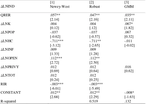
Table 2b reports the results obtained from the two estimation techniques for the industrial sector.
For the two OLS cases, the coefficient of the real exchange rate undervaluation term appears
positive and significant at the conventional levels of significance. The GMM technique also finds
real exchange rate undervaluation to impact on the industrial sector positively and significantly
at 5% level (sees Panel [3] of Table 2b). Similar to the results reported for the agricultural sector,
11
undervaluation index when compared to the GMM technique. More importantly, we can
[image:12.612.70.537.148.481.2]conclude that exchange rate undervaluation exerts a positive impact on the industrial sector.
Table 2b: Exchange Rate Undervaluation and Industrial Sector Performance
∆LNIND [1] Newey-West [2] Robust [3] GMM QRER ∆LNK ∆LNPOP ∆LNHC ∆LNINF ∆LNOPEN ∆LNPRIVY ∆LNTOT RIR CONSTANT R-squared .057** [2.14] .004 [0.12] -.037 [-0.62] -.711*** [-3.12] .009 [1.33] .112*** [2.72] .012 [0.69] .012 [0.24] -.003*** [-6.01] .012** [2.68] .047** [2.16] .004 [.12] -.037 [-0.57] -.711** [-2.65] .009 [1.28] .112** [2.50] .012 [0.64] .012 [0.25] -.003*** [-5.49] .012** [2.29] 0.519 .035** [2.11] .067* [1.82] .067 [0.32] -.011 [-0.02] .016 [0.62] -.008* [-1.63] .132
Note: *, **, *** indicate rejection of the null hypothesis at 10%, 5%, and 1%, respectively.Values in parenthesis denote t-statistics.
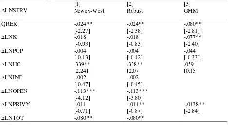
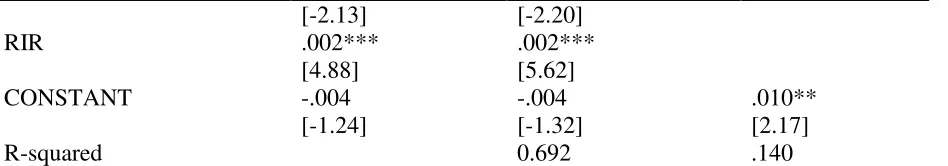
The impact of exchange rate undervaluation on service sector performance is shown in Table 2c.
In Panels [1] and [2], we report the results for the OLS technique using the Newey-West and
robust standard errors, respectively. The results here are quite contrasting to those reported
earlier for the agricultural and industrial sectors. Real exchange rate undervaluation negatively
and significantly impact on the performance of the service sector. This holds even after
12
A possible explanation of these results resides in the nature of outputs produced by these sectors.
The agricultural and industrial sectors of the South African economy usually produce outputs
that are exportable. It means that as the rand depreciates, other factors remaining the same,
outputs from these sectors become cheaper for external buyers. The external demand for goods
from these sectors will increase, thereby exerting upward pressure on prices of these goods,
which enhances the profitability, and production in these sectors.12 The World Bank, for
example, attributed the dismal agricultural sector performance in many African countries to their
overvalued currencies (see World Bank, 1984; Edwards, 1989).
Outputs produced in the service sector, in contrast, are mostly locally consumed. The inputs used
in this sector are, however, imported. This means that as the rand depreciates, inputs become
expensive. The producers of services will therefore try to cut costs on inputs by increasing the
prices of services, which will put downward pressure on domestic demand for services. Falling
demand for services will have negative implications for the production of services in the
economy. Therefore, real exchange rate undervaluation is expected to exert negative influence on
[image:13.612.69.537.437.698.2]service sector performance in South Africa.
Table 2c: Exchange Rate Undervaluation and Service Sector Performance
∆LNSERV [1] Newey-West [2] Robust [3] GMM QRER ∆LNK ∆LNPOP ∆LNHC ∆LNINF ∆LNOPEN ∆LNPRIVY ∆LNTOT -.024** [-2.27] -.018 [-0.93] -.004 [-0.13] .339** [2.24] -.002 [-0.47] -.113*** [-4.12] -.011 [-0.71] -.080** -.024** [-2.38] -.018 [-0.83] -.004 [-0.12] .338** [2.07] -.002 [-0.45] -.113*** [-3.80] -.011** [-0.87] -.080** -.080** [-2.81] -.077** [-2.40] -.044 [-0.33] .059 [0.15] -.0138** [-2.84] 12
13 RIR
CONSTANT
R-squared
[-2.13] .002*** [4.88] -.004 [-1.24]
[-2.20] .002*** [5.62] -.004 [-1.32] 0.692
.010** [2.17] .140
Note: *, **, *** indicate rejection of the null hypothesis at 10%, 5%, and 1%, respectively.Values in parenthesis denote t-statistics.
3.3 Sensitivity Analysis
The results presented earlier are based on the index of real exchange rate undervaluation
constructed using quantile regression. One critical question is whether these results would hold
when we use a different index to measure real exchange rate undervaluation. The answer to this
question has important policy implication. An affirmative response would mean that our earlier
findings would hold irrespective of how we analyze the problem. However, a contrary response
implies that our conclusion could be misleading. To be sure that our findings are not
questionable, we perform a sensitivity analysis of our main undervaluation index using an
alternative index. This index, as discussed earlier, is based on the HP filtering technique. In the
next few paragraphs, we discuss how the real exchange rate undervaluation measured in this
[image:14.612.70.544.72.155.2]sense affect the performance of the three sectors of the South African economy.
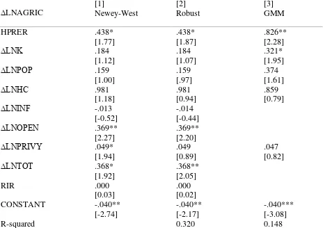
Table 3a reports the results of the impact of real exchange rate undervaluation (measured in the
HP filter sense) on the performance of the agricultural sector. Panels [1] and [2] show that the
real exchange rate undervaluation positively and significantly affects the performance of the
agricultural sector. The results hold when we controlled for endogeneity using the GMM
technique in Panel [3]. The results compare favorably with those obtained for the QRER index.
The difference is the size of the effect. Real exchange rate undervaluation has a relatively
moderate effect on agricultural sector performance when considered under the QRER. The
conclusion, however, still stands: real exchange undervaluation induces the performance of the
14
Table 3a: Alternative Measure of Undervaluation and Agriculture Sector Performance
∆LNAGRIC [1] Newey-West [2] Robust [3] GMM HPRER ∆LNK ∆LNPOP ∆LNHC ∆LNINF ∆LNOPEN ∆LNPRIVY ∆LNTOT RIR CONSTANT R-squared .438* [1.77] .184 [1.12] .159 [1.00] .981 [1.18] -.013 [-0.52] .369** [2.27] .049* [1.94] .368* [1.92] .000 [0.03] -.040** [-2.74] .438* [1.87] .184 [1.07] .159 [.97] .981 [0.94] -.014 [-0.44] .369** [2.20] .049 [0.89] .368** [2.05] .000 [0.02] -.040** [-2.17] 0.320 .826** [2.28] .321* [1.95] .374 [1.61] .859 [0.79] .047 [0.82] -.040*** [-3.08] 0.148
Note: *, **, *** indicate rejection of the null hypothesis at 10%, 5%, and 1%, respectively.Values in parenthesis denote t-statistics.
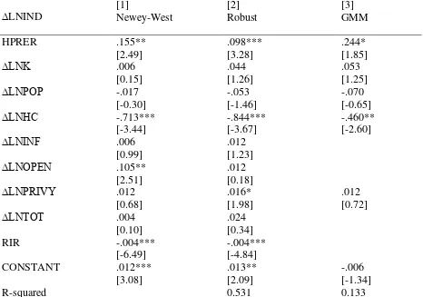
The estimates for the industrial sector when undervaluation is defined in terms of the HP filter
are shown in Table 3b. Panels [1], [2] and [3] report the results using the OLS and GMM
estimators, respectively. Here, real exchange rate undervaluation is found to exert a positive and
significant influence on the performance of the industrial sector. The estimated influence remains
valid after controlling for endogeneity (see Panel [3]). The results conforms to the ones we found
15
Table 3b: Alternative Measure of Undervaluation and Industrial Sector Performance
∆LNIND [1] Newey-West [2] Robust [3] GMM HPRER ∆LNK ∆LNPOP ∆LNHC ∆LNINF ∆LNOPEN ∆LNPRIVY ∆LNTOT RIR CONSTANT R-squared .155** [2.49] .006 [0.15] -.017 [-0.30] -.713*** [-3.44] .006 [0.99] .105** [2.51] .012 [0.68] .004 [0.10] -.004*** [-6.49] .012*** [3.08] .098*** [3.28] .044 [1.26] -.053 [-1.46] -.844*** [-3.67] .012 [1.23] .012 [0.18] .016* [1.98] .024 [0.34] -.004*** [-4.84] .013** [2.09] 0.531 .244* [1.85] .053 [1.25] -.070 [-0.65] -.460** [-2.60] .012 [0.72] -.006 [-1.34] 0.133
Note: *, **, *** indicate rejection of the null hypothesis at 10%, 5%, and 1%, respectively. Values in parenthesis denote t-statistics.
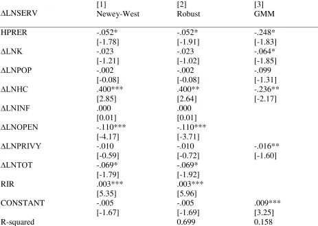
In Table 3c, we report the estimates for the service sector when the HPRER is used as our
measure of real exchange rate undervaluation. As with the previous tables, Panels [1], [2] and [3]
show the results obtained using the OLS and GMM estimators. The results indicate that real
exchange rate undervaluation exerts negative and significant influence on the service sector
performance. And this is true, even after controlling potential endogeneity. Note that the
estimated coefficient of the real exchange rate undervaluation term for this case appears slightly
16
Table 3c: Alternative Measure of Undervaluation and Service Sector Performance
∆LNSERV [1] Newey-West [2] Robust [3] GMM HPRER ∆LNK ∆LNPOP ∆LNHC ∆LNINF ∆LNOPEN ∆LNPRIVY ∆LNTOT RIR CONSTANT R-squared -.052* [-1.78] -.023 [-1.21] -.002 [-0.08] .400*** [2.85] .000 [0.01] -.110*** [-4.17] -.010 [-0.59] -.069* [-1.79] .003*** [5.35] -.005 [-1.67] -.052* [-1.91] -.023 [-1.02] -.002 [-0.08] .400** [2.64] .000 [0.01] -.110*** [-3.71] -.010 [-0.72] -.069* [-1.92] .003*** [5.96] -.005 [-1.69] 0.699 -.248* [-1.83] -.064* [-1.85] -.099 [-1.31] -.236** [-2.17] -.016** [-1.60] .009*** [3.25] 0.158
Note: *, **, *** indicate rejection of the null hypothesis at 10%, 5%, and 1%, respectively.Values in parenthesis denote t-statistics.
4. Concluding Remarks
Real exchange rate misalignment has been found to influence the performance of economies
around the globe. Some empirical studies find real exchange rate undervaluation to stimulate
economic performance, and overvaluation to hurt economic performance. Other empirical
studies simply admonished against any misalignment of the real exchange rate, arguing that real
exchange rate misalignments are not favourable for economic performance. Most recent studies,
however, side with the former conclusions (i.e. real exchange rate misalignments are crucial to
economic performance). The question is: through what channels does real exchange rate
undervaluation influence economic performance? This question has stimulated current empirical
and theoretical research. This paper sheds light on the channels through which real exchange rate
17
key contribution of our paper. In addition, we introduce two methods for constructing the index
of real exchange rate undervaluation, which differs from the ones found in the existing studies.
The first follow the approach used in Rodrik (2008) but departs from this author’s approach by
using the quantile regression estimator. The second measure of real exchange rate undervaluation
is the cyclical component of the real exchange rate obtained using the Hodrick-Prescott filter.
We decomposed the South African economy into three sectors, namely: agriculture, industry,
and service. Using the OLS and GMM estimation techniques; a time series data covering
1962-2014; and a standard regression model for each sector, we established two important results: (i)
real exchange rate undervaluation exerts a positive impact on economic performance by
enhancing agricultural and industrial sectors; and (ii) a negative impact on economic
performance by reducing the performance of the service sector. These results are found to be
robust to the measure of real exchange rate undervaluation we employed, serial correlation,
omitted variables heteroskedasticity, and potential endogeneity.
References
Balassa, B. (1964). The Purchasing Power Parity Doctrine: A Reappraisal. Journal of Political Economy 72: 584–96.
Barro, R., and Lee, J.-W. (2013). A New Data Set of Educational Attainment in the World, 1950-2010. Journal of Development Economics, 104, 184-198.
Beck, T., Demirgüç-Kunt, A., and Levine, R. (2000). A New Database on Financial Development and Structure. World Bank Economic Review 14: 597-605.
Bhagwati, J. N. (1984). Why Are Services Cheaper in The Poor Countries? The Economic Journal 94: 279–86.
Bhalla, S. S. (2007). Second Among Equals: The Middle Class Kingdoms of India and China, Peterson Institute of International Economics, Washington, DC, forthcoming (May 21, 2007 draft).
18
Edwards, S. (1989). Exchange Rate Misalignment in Developing Countries. World Bank Research Observer 4(1): 3-21.
Eichengreen, B. and Gupta, P. (2013). The real exchange rate and export growth: are services different ? Policy Research Working Paper Series 6629, The World Bank.
Elliott, G. R., Rothenberg, T. J., and Stock, J. H. (1996). Efficient Tests for an Autoregressive Unit Root. Econometrica 64: 813–836.
Fischer, S. (1993). The Role of Macroeconomic Factors in Growth. Journal of Monetary Economics 32: 485-512.
Gala, P. (2008). Real Exchange Rate Levels and Economic Development: Theoretical Analysis and Empirical Evidence. Cambridge Journal of Economics 32: 273–288.
Gluzmann, P., Levy-Yeyati, E., and Sturzenegger, F. (2007). Exchange Rate Undervaluation and Economic Growth: Díaz Alejandro (1965) Revisited, Unpublished Paper, John F. Kennedy School of Government, Harvard University, 2007.
Heston, A., Summers, R. and Aten, B. (2012). Penn World Table Version 7.1, Center for International Comparisons of Production, Income and Prices at the University of Pennsylvania. Available at: https://pwt.sas.upenn.edu/php_site/pwt_index.php. Accessed: 11/01/2015.
Hodrick, R., and Prescott, E. C. (1997). Postwar U.S. Business Cycles: An Empirical Investigation. Journal of Money, Credit, and Banking 29 (1): 1–16.
Johnson, S. H., Ostry, J. and Subramanian, A. (2007). The Prospects for Sustained Growth in Africa: Benchmarking the Constraints (March 2007). IMF Working Paper No. 07/52.
Newey, W. K., and West, K. D. (1987). A Simple, Positive Semi-Definite, Heteroskedasticity and Autocorrelation Consistent Covariance Matrix. Econometrica, 55: 703–708.
Officer, L. H. (1976). The Productivity Bias in Purchasing Power Parity: An Econometric Investigation. IMF Staff Papers 23: 545–79.
Phillips, P. C. B., and Perron, P. (1988). Testing for a Unit Root in Time Series Regression. Biometrika 75: 335–346.
Pick, D.H. and Vollrath, T.L. (1994). Real Exchange Rate Misalignment and Agricultural Export Performance in Developing Countries. Economic Development and Cultural Change, 42,3,555-571.
19
Ravn, M., and Uhlig, H. (2002). On Adjusting the Hodrick-Prescott filter for the Frequency of Observations. The Review of Economics and Statistics, Vol. 84 (2): 371-375.
Razin, O., and Collins, S. M. (1997). Real Exchange Rate Misalignments and Growth, Georgetown University.
Rodrik, D. (2008). The Real Exchange Rate and Economic Growth, Working Paper, John F. Kennedy School of Government, Harvard University, Cambridge, MA 02138, Revised, September 2008.
Samuelson, P. A. (1964). Theoretical Notes on Trade Problems. Review of Economics and Statistics 46: 145–54.
Vieira, F. V. and MacDonald, R. (2012). A Panel Data Investigation of Real Exchange Rate Misalignment and Growth. Estudios de Economia 42(3): 433—456.
Wang, K-L., and Barrett, C. B. (2007). Estimating the Effects of Exchange Rate Volatility on Export. Journal of Agricultural and Resource Economics, 32(2): 225-255.
Whittaker, E. T. (1923). On a New Method of Graduation. Proceedings of the Edinburgh Mathematical Association, Vol. 41: 63-75.
World Bank. (1984). Toward-Sustained Development in Sub-Saharan Africa. Washington, D.C.
20
[image:21.612.76.548.100.410.2]Appendix A
Figure 1: Plot of the Exchange Rate Undervaluation Indexes
Note: qrer = real exchange rate undervaluation index constructed using quantile regression; hprer = real exchange rate undervaluation index constructed using HP filter. Clearly, the indexes are very similar over the period 1962-2014.
-.
2
0
.2
.4
.6
1962 1967 1972 1977 1982 1987 1992 1997 2002 2007 2012
year
21
Technical Appendix
The Hodrick-Prescott Filter
The Hodrick-Prescott (HP) filter is a filtering technique mostly utilized in empirical
macroeconomics to filter a time series variable into its cyclical and trend components. Whittaker
(1923) first developed this technique. However, it was made popular as an empirical tool in the
seminal paper of Hodrick and Prescott (1997). The main importance of the HP filter is its ability
to generate a smooth-curve representation of a time series, which is susceptible to long-run
impacts than cyclical fluctuations.
The HP filter builds on the idea that a time series variable, say 𝑥𝑡, can be filtered into a trend (𝜏𝑡)
and cyclical component (𝑐𝑡). Suppose that 𝑥𝑡 = 𝜏𝑡+𝑐𝑡+𝜇𝑡, where 𝜇𝑡 is the error term of the
time series variable at time t. Then, there exist a positive value of a multiplier 𝜆, such that 𝜏
solves the minimization problem:
min
𝜏 ��(𝑥𝑡− 𝜏𝑡)2+𝜆 �[(𝜏𝑡+1− 𝜏𝑡)−(𝜏𝑡− 𝜏𝑡−1)]2 𝑇−1
𝑡=2 𝑇
𝑡=1
�
where the sum of the squared deviations 𝑑𝑡 =𝑥𝑡− 𝜏𝑡 penalizes the short-run fluctuations in the
time series. The second term is a multiple of the multiplier (𝜆) and the sum of squares of the
second differences in the trend component of the series. This term penalizes deviations in the
growth of the trend component of the time series. Higher values of 𝜆 imply higher penalties. For
quarterly data, Hodrick and Prescott (1997) recommend that we set 𝜆=1600. Ravn and Uhlig
(2002) recommend that we choose 𝜆 = 6.25 and 129600 for annual and monthly data,