Government Commitment and Unemployment Insurance Over the Business Cycle

Munich Personal RePEc Archive

Government Commitment and

Unemployment Insurance Over the

Business Cycle

Pei, Yun and Xie, Zoe

State University of New York at Buffalo, Federal Reserve Bank of

Atlanta

3 November 2016

Government Commitment and Unemployment Insurance

over the Business Cycle

Yun Pei †

State University of New York at Buffalo

Zoe Xie ‡

Federal Reserve Bank of Atlanta

Abstract

We investigate the role of government commitment to future policies in shaping unemployment insurance (UI) policy in a stochastic general equilibrium model of labor search and matching. Compared with the optimal (Ramsey) policy of a government with commitment, the policy under no commitment characterized by a Markov-perfect equilibrium has higher benefits and leads to higher unemployment rates in the steady state. We also find starkly different policy responses to a productivity shock or changes in unemployment. The differences arise because the Ramsey government can use an ex-ante committed policy to stimulate job search.

Keywords: Unemployment insurance, Commitment, Markov-perfect equilibrium, Business cycle JEL classifications: E61, J64, J65, H21

∗_{This version: November 3, 2016. First draft: July 2015. The views expressed here are the opinions of the authors} only and do not necessarily represent those of the Federal Reserve Bank of Atlanta or the Federal Reserve System.

†_{Department of Economics, State University of New York at Buffalo, 415 Fronczak Hall, Buffalo, NY 14260. Email:} yunpei@buffalo.edu.

1

Introduction

A recent literature finds that the optimal (Ramsey) unemployment insurance (UI) policy is more generous at the start of a recession and less generous as the recession gets more severe to induce a recovery.1 This pattern differs from the movement of benefits in the U.S. over the business cycle. In particular, benefits are more generous the deeper the recession gets as measured by unemployment.2 In addition, Congress voted frequently on extending UI benefits from 2008 to 2013 during the Great Recession, which reflects the government’s lack of commitment over UI policies. In this paper, we argue that when the government cannot commit to a prescribed path of benefit policies, it cannot use UI policy to induce recovery in recessions. Such a policy more closely resembles the U.S. policy. We characterize and compare the benefit policies with and without commitment and study its impact on the labor market.

The model integrates risk-averse workers and endogenous search intensity by unemployed workers into the Diamond-Mortensen-Pissarides framework, with business cycle driven by shocks to aggregate labor productivity. Three types of entities inhabit the model economy: workers, firms and govern-ment. Employed workers work for firms and get paid wages. Unemployed workers receive UI benefits and choose how much to search. Job search incurs utility cost, but also increases the probability that an unemployed worker finds a job. Firms matched with workers produce and pay workers wage, while unmatched firms post job vacancies at a fixed cost. Wages are determined through a Nash bargaining process.

Because the focus of the present paper is on the comparison between UI policies with and without government commitment, we abstract from the distinction between benefit level and the expected duration that an unemployed worker can receive benefits (“benefit duration”) and instead use the benefit level alone to capture the generosity of UI policies. The government chooses UI benefits financed by a non-distortionary tax. More generous futureUI benefits reduce unemployed worker’s current search intensity. Through general equilibrium effects, higher benefits reduce firm’s vacancy posting by increasing worker’s outside option in the wage bargaining process.

We compare two economies. In the first economy, the optimal state-contingent UI policy is the solution to a Ramsey problem of the government, which takes competitive equilibrium conditions as constraints. Because the government can commit to future policies, it optimally chooses the level of UI benefits for all periods of time and for all possible realizations of productivity shocks. The Ramsey policy, however, is not time consistent. In particular, the current government would like to reduce promised future benefitsbefore unemployed workers choose how much to search (“ex-ante policy”), and increase benefits after they have chosen job-search level (“ex-post policy”).3 _Because

1_{See, for example,Jung and Kuester(2015) andMitman and Rabinovich(2015).}

2 _{By generosity we refer loosely to either an increase in the benefit level received by unemployed workers or the} potential duration that a benefit-eligible unemployed worker can stay on benefits.

the government wants to implement different policies ex-ante and ex-post, such a policy is time inconsistent and cannot be implemented without government commitment.

In the second economy, we characterize and solve for the time-consistent UI policy. We use the concept of Markov-perfect equilibrium, à la Klein, Krusell and Ríos-Rull (2008). Each period the government chooses current policies to maximize current and future welfare, taking as given future government’s policy rules. Because the Markov government only chooses policies for the current period, its policies differ from the Ramsey policies. First, it does not consider how its policies affect private-sector choices in the previous period, whereas the Ramsey government internalizes this effect. Second, the Markov government can only indirectly influence future polices through the states of the economy, while the Ramsey government predetermines a full sequence of state-contingent policies at time 0.

We calibrate the model to match the U.S. economy. Using these calibrated parameters, we then compute the Ramsey and the Markov policies. Overall, the Markov economy has more generous UI benefits, lower search intensity, lower job postings and higher unemployment rate than the Ramsey economy. This is not surprising, given that the Markov government has no commitment and chooses more generous benefits. This highlights the importance of commitment.

An important result concerns the dynamic responses of different governments. The Ramsey UI benefits decrease when current labor productivity is higher or unemployment rate is higher, whereas the Markov UI benefits increase when current labor productivity is higher but does not change much with respect to unemployment rate. The intuition is that the optimal (Ramsey) benefits are lower in states of the economy where the marginal social benefit of job creation is higher, because lower benefits encourage job search and vacancy posting. The marginal social benefit of job creation is higher when productivity is higher, because each worker-firm pair produces higher output; it is also higher when unemployment is higher, because the probability of filling a job is higher. The Markov government considers the previous period bygone, and so it does internalize these social gains. Instead, the Markov government increases UI benefits when productivity is high, because higher wages (increase in productivity shared between workers and firm) increase the gain from redistribution. When unemployment is higher, the incentive to encourage search is higher, but there is also a larger gain from providing insurance. These two effects cancel each other out, and the Markov benefits vary little with respect to unemployment rate.

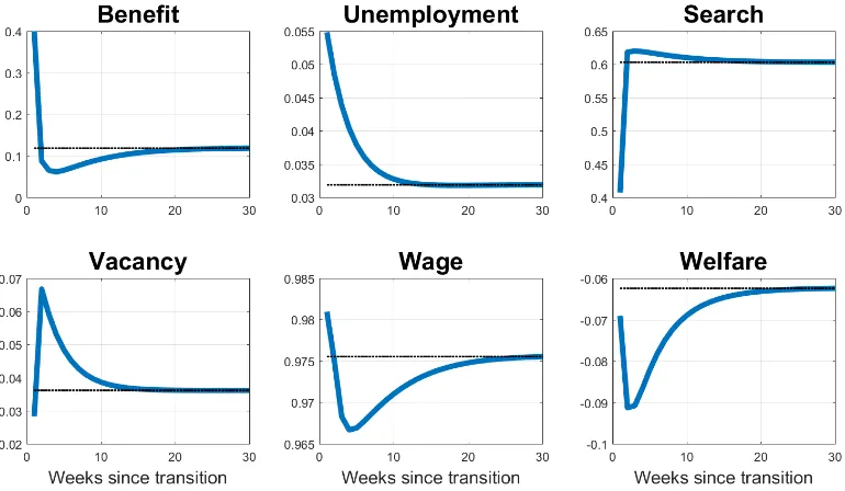
As the economy recovers, the Markov government gradually increases benefits to the pre-shock level. The richer dynamics of the optimal policy reflects the benefit of commitment—because the Ramsey government has commitment over future policies, it can use temporary changes in the UI policy to smooth consumption over the business cycle. As a result, the Ramsey economy experiences relatively fast recovery in unemployment, while the Markov economy undergoes a much slower recovery.

Several simplifying assumptions are made for tractability. First, neither workers nor government can save or borrow. Allowing workers to save will reduce the cyclical responses of both Ramsey and Markov governments as savings provide self-insurance. If government can save or borrow, there will be larger cyclical responses as the government is not constrained by budget constraints every period. Both assumptions, however, will not affect the comparison of the Ramsey and Markov policies. Second, the Markov government in our setup makes decision every period. Given the weekly frequency, it means that the government makes UI policy decisions every week in our setup, which is much more frequent than in reality. Changing model frequency to quarterly, however, will be a departure from the standard frequencies used in analysis of the labor market.

A review of the related literature and our contributions to the literature is given next.

1.1

Related literature

This paper is closely related to two strands of literature: the literature on UI and the literature on time-consistent public policy.

The literature on UI dates back to Mortensen (1977), who argues that unemployment insurance reduces job search effort by the unemployed. Since Mortensen, the majority of this literature takes one of two approaches: either studying the effects of actual UI policy or looking for an optimal policy. The present paper aims to bridge the two approaches by endogenizing government choice of UI policy. Here we take the stance that the government, when making UI policies, is unable to commit to future policies.

One of the classic empirical results in public finance is that social insurance programs such as UI reduce labor supply. Earlier works include Moffitt (1985) and Meyer (1990), who show that a 10% increase in unemployment benefits raises average unemployment durations by 4–8% in the U.S.Krueger and Meyer (2002) and Gruber (2007), for example, interpret this finding as evidence that UI has significant moral hazard costs. Our framework relies on a similar mechanism. When the

expected payoff from unemployment is high relative to future wages, unemployed workers search less

actively. Chodorow-Reich and Karabarbounis(2015) construct a time series of the opportunity cost of employment and find that the cost is procyclical and volatile over the business cycle.

tighter liquidity constraints. Because this “liquidity effect” has the socially beneficial effect of cor-recting credit market failure, the truly optimal benefit level, as Chetty (2008) argues, should be higher than if such an effect were ignored. For tractability, the present paper abstracts from the credit market and therefore cannot directly control for the liquidity effect.

The literature on optimal UI has traditionally adopted a principal-agent framework (e.g., Hopen-hayn and Nicolini 1997,Wang and Williamson 2002,Shimer and Werning 2007,2008, and Golosov, Maziero and Menzio 2013). This framework allows moral hazard frictions to be characterized in a steady state, but it becomes intractable when extended to a business cycle environment. The lit-erature typically shows that the optimal benefit should decline with the unemployment duration of an individual worker. For tractability, our paper abstracts from duration-dependent benefits. More recently,Mitman and Rabinovich (2015) study optimal benefits over the business cycle in a search-matching framework with endogenous unobservable search intensity. Jung and Kuester (2015) take a more general approach by studying the optimal mix of unemployment benefits, hiring subsidies, and layoff taxes in a recession. These papers assume that the government is able to commit to future policies. Although this assumption is innocuous and standard for normative analysis, such policies are time inconsistent and thus hardly implementable without government commitment. Our paper complements the literature by characterizing a time-consistent UI policy. Intuitively, the Ramsey government wants people to search hard in normal times when unemployment is low and the marginal return to search is high. To this end, the Ramsey government promises less generous benefits during recessions.

The current paper is also related to the literature on time-consistent public policy (see, e.g., Alesina and Tabellini 1990, Chari and Kehoe 2007, Battaglini and Coate 2008, and Yared 2010).4 Methodologically, our paper followsKlein, Krusell and Ríos-Rull(2008) to characterize the Markov-perfect equilibrium of a dynamic game in terms of a generalized Euler equation (GEE). Whereas Klein, Krusell and Ríos-Rull (2008) focus on a deterministic economy, we are interested in how government policy responds to business cycle fluctuations. Recent applications of Markov-perfect equilibrium includeSong, Storesletten and Zilibotti(2012), who study intergenerational conflict over debt in a politico-economic environment.

The rest of the paper proceeds as follows. Section 2 describes the model environment and defines the private-sector competitive equilibrium. Section 3 presents the government’s problem first as an optimal policy problem, and then as part of a Markov-perfect equilibrium. We characterize the solutions and solve both government’s problems in this section. Section 4 describes the calibration strategy. Section 5 presents the quantitative results. Section 6 concludes. We relegate all derivations and additional figures to the Appendix.

2

Model

In this section, we describe the model environment and characterize the competitive equilibrium. Similar toMitman and Rabinovich(2015), we use a Diamond-Mortensen-Pissarides framework with aggregate productivity shocks to model the private sector.5

2.1

Model environment

Time is discrete and infinite. The model is inhabited by a mass of infinitely lived workers and firms. The measure of workers is normalized to one. In any given period, a worker can be either employed or unemployed. Workers are risk-averse and maximize expected lifetime utility given by

E₀ ∞

∑︁

𝑡=0

Ñ𝑡𝑈(𝑐𝑡,𝑠𝑡)

whereE_{0is the period-0 expectation factor,Ñ is the time discount factor. Period utility𝑈(𝑐,𝑠)takes}

consumption of goods 𝑐 and search intensity 𝑠 as inputs. Utility is increasing in 𝑐 and decreasing in 𝑠. Only unemployed workers supply positive search intensity, i.e. there is no on-the-job search. Each period, an employed worker gets paid wage from production. Wages are determined through a canonical bargaining process to be specified later in the section. An unemployed worker receives unemployment benefits 𝑏. In addition, an unemployed worker also producesℎ, which we take as the combined value of leisure, home production and welfare. There are no private insurance markets and workers cannot save or borrow.

Firms are risk neutral and maximize the expected discounted sum of profits, with the same discount factor Ñ. A firm can be either matched to a worker (and producing) or vacant. A vacant firm posting a vacancy incurs a flow cost Ù.

Unemployed workers and vacancies form new matches. Let 𝑢 and 𝑣 denote the measure of unemployed worker, and the measure of vacancies posted, respectively. Then the number of new matches formed in a period is given by the matching function 𝑀(𝑠𝑢,𝑣), where the quantity 𝑠𝑢 is the measure of efficiency units of search by the unemployed in the economy. The matching function exhibits constant returns to scale, is strictly increasing and strictly concave in both arguments, and is bounded above by the number of potential matches : 𝑀(𝑠𝑢,𝑣)⊘min¶𝑠𝑢,𝑣♢. The job-finding probabilities per efficiency unit of search intensity, 𝑓, and the job-filling probability per vacancy,𝑞,

are functions of labor market tightness, 𝜃=𝑣/(𝑠𝑢). More specifically,

𝑓(𝜃) = 𝑀(𝑠𝑢,𝑣)

𝑠𝑢 =𝑀(1,𝜃) 𝑞(𝜃) = 𝑀(𝑠𝑢,𝑣)

𝑣 =𝑀

⎤₁

𝜃, 1

⎣

Following the assumptions made on 𝑀, 𝑓(𝜃) is increasing in 𝜃 and 𝑞(𝜃) is decreasing in 𝜃. The job finding probability for an unemployed searching with intensity𝑠is 𝑠𝑓(𝜃). Existing matches are destroyed exogenously with constant job separation probabilityÓ.

Only a matched pair of a worker and a firm can produce. Each matched pair produces 𝑧, where

𝑧 is the aggregate labor productivity. 𝑧is constant 𝑧¯ in the steady state, and time-varying 𝑧𝑡 in the

economy off steady-state.

2.2

Government

The government cannot borrow or lend; instead it balances budget each period. The government finances unemployment benefits 𝑏 through a lump sum tax, á, on all workers, both employed and unemployed.6 _{The government budget constraint is}

(1) á =𝑢𝑏

The government decides on the generosity of the unemployment insurance program by varying benefit level, 𝑏⊙0. Once a benefit level is determined, all unemployed workers receive the same benefit in that period. This way of modeling the unemployment insurance system is a simplification of the reality where not all unemployed workers receive benefits. This assumption is common in the literature, for example, Landais, Michaillat and Saez (2010) and Jung and Kuester (2015) both assume all unemployed receive benefits. The advantage of this setup is reduced computational complexity while still allowing the generosity of the unemployment insurance program to change. The unemployment benefits here can be thought of as compounding the potential duration and level of unemployment benefits.7

2.3

Timing

The timing of events within a period is illustrated in Figure1and is as follows. The economy enters a period 𝑡 with a level of unemployment 𝑢. The aggregate shock 𝑧 then realizes. (𝑧,𝑢) are the

6 _{We experiment with alternative tax structure where either only employed workers pay tax, or only firms pay tax} (in the form of a lump sum tax on profits). Results are not presented in the paper but are available upon request.

(𝑧,𝑢)

𝑡 _{policy(𝑏,á)} production, consumption

search, vacancy posting

𝑢′

𝑧′ 𝑡+1

Figure 1: Timing of events.

aggregate states of the economy. Government policies(𝑏,á)for the period are known to workers and firms.

Employed workers produce 𝑧 and receive a bargained wage 𝑤. Unemployed workers produce ℎ

and receive benefits𝑏. All workers pay a lump sum taxá out of wage or benefit.

Given aggregate states and government policies for the period, unemployed workers choose search intensity 𝑠. At the same time, firms decide how many vacancies to post, at cost Ùper vacancy. The aggregate search is then 𝑠𝑢, and the market tightness is equal to 𝜃 =𝑣/(𝑠𝑢). The fraction of unemployed workers who find jobs is 𝑓(𝜃)𝑠. At the same time, a fraction Ó of the existing 1⊗𝑢

matches are exogenously destroyed. The law of motion of unemployed workers is

(2) 𝑢′=Ó(1⊗𝑢) + (1⊗𝑓(𝜃)𝑠)𝑢

2.4

Workers

Denote by 𝑔 the government policy (𝑏,á). Because we abstract from household savings and all unemployed workers receive unemployment benefits, a worker entering a period unemployed consumes

ℎ+𝑏. He also chooses search intensity 𝑠. With probability 𝑓(𝜃(𝑧,𝑢;𝑔))𝑠, he finds a job and starts working the following period. Let 𝑉𝑒(𝑧,𝑢;𝑔) and 𝑉𝑢(𝑧,𝑢;𝑔) be the values of an employed and an unemployed worker, respectively, with the beginning-of-period unemployment 𝑢 and realized aggregate shock 𝑧, given government policy for that period 𝑔= (𝑏,á). An unemployed worker’s optimization problem is

𝑉𝑢(𝑧,𝑢;𝑔) = max

𝑠 𝑈(𝑐,𝑠) +Ñ𝑓(𝜃(𝑧,𝑢;𝑔))𝑠

E_𝑉𝑒_(𝑧′_,𝑢′_;𝑔′_{) +Ñ(1⊗𝑓(𝜃(𝑧,𝑢;𝑔))𝑠)}E_𝑉𝑢_(𝑧′_,𝑢′_;𝑔′₎

(3)

A worker entering a period employed produces and consumes his wage𝑤. With probabilityÓ, he loses his job and becomes unemployed the following period. There is no intra-temporal search, so a newly separated worker remains unemployed for at least one period. The Bellman equation of an employed worker is then

𝑉𝑒(𝑧,𝑢;𝑔) = 𝑈(𝑤(𝑧,𝑢;𝑔), 0) +Ñ(1⊗Ó)E_𝑉𝑒_(𝑧′_,𝑢′_;𝑔′_{) +ÑÓ}E_𝑉𝑢_(𝑧′_,𝑢′_;𝑔′₎

(4)

is taken to be constant through time.

2.5

Firms

In order to be matched with a worker and produce, a firm posts a vacancy.8 A firm that posts a vacancy incurs a flow cost Ù. With probability 𝑞(𝜃(𝑧,𝑢;𝑔)), a vacancy is filled and ready for production the following period. Let𝐽𝑢_{(𝑧,𝑢;𝑔)be the value of an unmatched firm posting a vacancy.}

The Bellman equation of an unmatched firm is

𝐽𝑢(𝑧,𝑢;𝑔) = ⊗Ù+Ñ𝑞(𝜃(𝑧,𝑢;𝑔))E_𝐽𝑒_(𝑧′_,𝑢′_;𝑔′_{) +Ñ(1⊗𝑞(𝜃(𝑧,𝑢;𝑔)))}E_𝐽𝑢_(𝑧′_,𝑢′_;𝑔′₎

(5)

where𝐽𝑒(𝑧,𝑢;𝑔) is the value of a matched firm. In equilibrium, under free-entry condition, the firm will post vacancies𝑣(𝑧,𝑢;𝑔)until 𝐽𝑢(𝑧,𝑢;𝑔) =0.

A matched firm receives output net of wages𝑧⊗𝑤(𝑧,𝑢;𝑔). With constant probabilityÓ, a match is destroyed at the end of period. The Bellman equation of a matched firm is

𝐽𝑒(𝑧,𝑢;𝑔) = 𝑧⊗𝑤(𝑧,𝑢;𝑔) +Ñ(1⊗Ó)E_𝐽𝑒_(𝑧′_,𝑢′_;𝑔′_{) +ÑÓ}E_𝐽𝑢_(𝑧′_,𝑢′_;𝑔′₎

(6)

2.6

Wage determination

Vacant jobs and unemployed workers are randomly matched each period according to the aggregate matching function𝑀(𝑠𝑢,𝑣). A realized match produces some economic rent that is shared between the firm and the worker through Nash bargaining. The assumption of Nash bargaining allows com-parison with the literature. We assume that wages are set period by period, so equilibrium wages respond to the state of the economy.

Worker’s surplus is the difference between the values of working at wage𝑤and being unemployed and receiving benefit𝑏. As a result, higher benefits increase worker’s surplus, and tends to drive up bargained wage. Firm’s surplus is the difference between the value of a match and that of running a vacancy. As explained before, vacant firm posts vacancies until its value is zero. Thus, the firm’s outside option is zero in equilibrium.

In particular, wage is chosen to maximize a weighted product of the worker’s surplus and the firm’s surplus when the state of the economy is (𝑧,𝑢) and government policy is 𝑔= (𝑏,á). The worker-firm pair thus solves

max

𝑤

⎤

𝑉𝑒(𝑧,𝑢;𝑔)⊗𝑉𝑢(𝑧,𝑢;𝑔)

⎣Õ⎤

𝐽𝑒(𝑧,𝑢;𝑔)⊗𝐽𝑢(𝑧,𝑢;𝑔)

⎣1⊗Õ

(7)

whereÕ∈(0, 1)is the bargaining power of the worker. 𝑉𝑒(𝑧,𝑢;𝑔)⊗𝑉𝑢(𝑧,𝑢;𝑔)is the worker’s surplus,

and 𝐽𝑒(𝑧,𝑢;𝑔)⊗𝐽𝑢(𝑧,𝑢;𝑔) is the firm’s surplus from the match. The solution to this bargaining problem, denoted𝑤(𝑧,𝑢;𝑔), is a function of the economy’s states.

2.7

Competitive equilibrium

Definition1. (competitive equilibrium) Given a policy𝑔= (𝑏,á)and an initial condition(𝑧⊗,𝑢⊗), a

competitive equilibrium consists of (𝑧,𝑢)- measurable functions for wages𝑤(𝑧,𝑢;𝑔), worker’s search intensity 𝑠(𝑧,𝑢;𝑔), market tightness 𝜃(𝑧,𝑢;𝑔), unemployment rate 𝑢′(𝑧,𝑢;𝑔), and value functions

𝑉𝑒(𝑧,𝑢;𝑔),𝑉𝑢(𝑧,𝑢;𝑔),𝐽𝑒(𝑧,𝑢;𝑔),𝐽𝑢(𝑧,𝑢;𝑔)such that for all(𝑧,𝑢;𝑔)

• the value functions satisfy the worker and firm Bellman equations (3)-(6)

• the search intensity 𝑠solves the unemployed worker’s maximization problem of (3) • the market tightness𝜃 is consistent with the free-entry condition, 𝑉𝑢(𝑧,𝑢;𝑔) =0 • the wage 𝑤solves the maximization problem of (7)

• unemployment satisfies the law of motion equation (2)

2.8

Characterization

The competitive equilibrium can be characterized by three optimality conditions.9 _{Appendix A} contains derivation of the optimality conditions. In what follows, primes denote variables of the following period, and subscripts denote derivatives.

The optimal choice of search intensity 𝑠for the unemployed worker is characterized by

⊗𝑈𝑠(ℎ+𝑏⊗á,𝑠)

𝑓(𝜃) = ÑE

⎦

𝑈(𝑤′⊗á′, 0)⊗𝑈(ℎ+𝑏′⊗á′,𝑠′) + (1⊗𝑓(𝜃′)𝑠′⊗Ó)⊗𝑈𝑠(ℎ+𝑏

′_⊗á′_,𝑠′₎

𝑓(𝜃′₎

⎢ (8)

The worker’s optimality condition states that the marginal cost (left-hand side) of increasing the job finding probability equals the marginal benefit (right-hand side). The marginal cost is the marginal disutility of search of the unemployed worker weighted by the aggregate job finding rate per efficiency unit of search. The marginal benefit is the sum of utility gain from being employed next period and the benefit of economizing on future search cost. A higher future benefit𝑏′ reduces the utility gain from being employed the next period, and thus lowers the marginal benefit of search today.

From firm’s free-entry condition

Ù

𝑞(𝜃) = ÑE

⎦

𝑧′⊗𝑤′+ (1⊗Ó) Ù

𝑞(𝜃′₎

⎢

(9)

where the marginal cost (left-hand side) equals the marginal benefit (right-hand side) of a filled vacancy. The marginal cost is the flow cost of posting a vacancy weighted by the probability of filling that vacancy. The marginal benefit is the profits from employing a worker. Because a newly formed match does not become operational until the next period, the benefit from production only has components from the next period.

Finally, Nash bargaining implies a relationship between the worker’s surplus from being employed and the firm’s surplus from hiring a worker.

[︁

𝑈(𝑤⊗á, 0)⊗𝑈(ℎ+𝑏⊗á,𝑠) + (1⊗𝑓(𝜃)𝑠⊗Ó)⊗𝑈s(ℎ+𝑏⊗á,𝑠)

𝑓(𝜃)

]︁

/𝑈𝑐(𝑤⊗á, 0)

𝑧⊗𝑤+ (1⊗Ó) Ù 𝑞(𝜃)

= Õ

1⊗Õ

The left-hand side of the equation is the ratio of worker’s to firm’s surplus weighted by marginal utility of higher wage. The worker’s surplus (top part) comes from utility gain of of being employed and reduced search cost (employed worker searches zero). Because workers are risk-averse, changes in wages have non-linear effect on his utility, as represented by𝑈𝑐(𝑤⊗á, 0). The firm’s surplus (bottom

part) derives from profit and reduced vacancy posting cost (producing firm posts zero vacancy). The right-hand side of the equation is the ratio of the worker’s to firm’s bargaining power. Equilibrium wage then equates the weighted ratio of worker/firm surplus to the ratio of their respective bargaining power.

Rearranging terms into a more compact condition for the equilibrium wage

(10)

Õ𝑈c(𝑤−á, 0)

⎦

𝑧−𝑤+ (1−Ó) Ù

𝑞(𝜃) ⎢

= (1−Õ) ⎦

𝑈(𝑤−á, 0)−𝑈(ℎ+𝑏−á,𝑠) + (1−𝑓(𝜃)𝑠−Ó)−𝑈s(ℎ+𝑏−á,𝑠) 𝑓(𝜃)

⎢

A higher future benefit𝑏′ lowers worker’s surplus. Given the future Nash bargaining condition, next period’s workers demand higher wage 𝑤′, and thus firm’s surplus is lower in equilibrium. The free-entry condition of (9) then implies a lower 𝜃, and thus a lower job-finding rate per efficiency search unit 𝑓(𝜃).

A contemporaneous decrease in the aggregate labor productivity 𝑧reduces firm’s surplus in (10) and as a result wages fall. Because current wage and productivity do not enter worker’s and firm’s optimality conditions (8)-(9), the contemporaneous fall in 𝑧 does not directly affect search or job-finding rate. Now consider a fall in the expected future productivity 𝑧′. In this latter case, firm reduces vacancy posting since expected return to future production is lower. Worker reduces search intensity, both because fewer vacancies lead to lower per-search-unit job-finding probability, and because lower expected aggregate productivity implies lower expected future wages.

3

Government Policies

In this section, we describe how a Ramsey government and a Markov government choose their poli-cies, respectively. To highlight the key difference between these two types of governments, we first illustrate the time inconsistency of the Ramsey policy using a simple example. We then describe the full Ramsey and Markov problems. We assume both governments are utilitarian planners, who maximize the expected value of the worker’s utility. Both governments have the same policy instru-ments, which are unemployment benefit𝑏 and taxá. However, the Ramsey government can commit to future policies, while the Markov government does not have the ability to commit. In the last subsection, we discuss the role of commitment.

3.1

A simple example to illustrate time inconsistency

Before describing the full Ramsey problem, we consider a simple example to illustrate the presence of time inconsistency in the Ramsey problem. There are two periods and a unit measure of workers. Workers search in the first period and consume in the second period. Assume no time discounting and firms. In the first period, 1⊗𝑢¯ of workers are guaranteed a job in the second period. The remaining 𝑢¯ workers choose whether to search, 𝑠∈ ¶0, 1♢, for a job starting in the second period. Search incurs utility cost of𝑐¯. Worker’s utility of consumption is given by𝑈(𝑐).

If the worker searches (𝑠=1), with probability 𝑓 he finds a job and receives wage𝑤¯ =1 in the second period; otherwise he receives unemployment benefit 𝑏⊘𝑤¯. Optimally the worker searches is and only if 𝑈(𝑤¯)⊗𝑈(𝑏)⊙𝑐¯/𝑓. The number of unemployed workers in the second period is

𝑢= (1⊗𝑓 𝑠)𝑢¯.

Government in this economy chooses 𝑏∈ ¶𝑏¯,𝑏♢at the beginning of period 1 to maximize average utility

𝑊 = (1⊗𝑢)𝑈(𝑤¯) +𝑢𝑈(𝑏)⊗𝑢¯1_𝑠=1𝑐¯

subject to 𝑢 = (1⊗𝑓 𝑠)𝑢¯

𝑠=1 iff𝑈(𝑤¯)⊗𝑈(𝑏)⊙𝑐¯/𝑓

Assume linear utility functions and𝑤¯⊗𝑏⊙𝑐¯/𝑓+ [¯𝑏⊗𝑏]/𝑓 (Ass1) so that𝑏=𝑏,𝑠=1.10 _Essentially, the government is choosing between

𝑊(𝑏=𝑏,𝑠=1) = [1⊗(1⊗𝑓)𝑢¯]𝑤¯ + (1⊗𝑓)𝑢𝑏¯ ⊗𝑢¯𝑐¯

𝑊(𝑏=𝑏¯,𝑠=0) = (1⊗𝑢¯)𝑤¯ +𝑢¯𝑏¯

Then by assumption (Ass1)𝑊(𝑏=𝑏,𝑠=1)> 𝑊(𝑏=¯𝑏,𝑠=0), and the government optimally chooses

𝑏*=𝑏,𝑠*=1,𝑢*= (1⊗𝑓)𝑢¯.

Now suppose the government can revise benefit after workers have chosen 𝑠. Then the ex-post optimal policy isˆ𝑏=𝑏¯, withex-postaverage utility given by𝑊(𝑏ˆ=𝑏¯,𝑠=1) = (1⊗𝑢*)𝑤¯+𝑢*𝑏¯⊗𝑢¯𝑐 >¯

𝑊(𝑏=𝑏,𝑠=1). The fact that there exists a better policyex-postillustrates the time inconsistency in this setup; time inconsistency, in turn, means lack of commitment leads to different policy outcomes than an economy with government commitment.

3.2

Ramsey government

In this section, we set up the full Ramsey problem. The modeling of the Ramsey government is very similar to that in Mitman and Rabinovich (2015). Since the Ramsey government has commitment to all its future policies at the beginning of time, the government’s decision problem is therefore to choose a sequence of unemployment benefits and taxes ¶𝑏𝑡,á𝑡♢∞𝑡=0 in order to maximize the worker’s

utility, taking into account how the private sector will respond to these policies. At time 0, the government decides on its policies for all future periods and for all possible realizations of shocks. The private sector takes government policies as given and follows the timing described in Section 2.

To reduce the number of policy instruments in the government’s problem, we use the following function derived from the government’s budget constraint to express tax

𝒯(𝑢,𝑏):=𝑢𝑏.

Then the government’s problem can be equivalently written as one of choosing policies ¶𝑏𝑡♢∞𝑡=0,

and allocation and prices ¶𝑤𝑡,𝑠𝑡,𝜃𝑡,𝑢𝑡+1♢∞𝑡=0 to maximize utility subject to the government budget

constraint and competitive equilibrium conditions.11 _{Formally, thegovernment period return function} at time𝑡 is given by 𝑅(𝑢𝑡,𝑏𝑡,𝑤𝑡,𝑠𝑡) = (1⊗𝑢𝑡)𝑈(𝑤𝑡⊗ 𝒯(𝑢𝑡,𝑏𝑡), 0) +𝑢𝑡𝑈(ℎ+𝑏𝑡⊗ 𝒯(𝑢𝑡,𝑏𝑡),𝑠𝑡).

Definition 2. (Ramsey policy) Given an initial unemployment rate 𝑢0 and aggregate labor

pro-ductivity𝑧0, the optimal government policy with commitment consists of a sequence of benefits and

taxes¶𝑏𝑡♢∞𝑡=0 that solves

max

¶𝑏t,𝑤t,𝑠t,𝜃t,𝑢t+1♢∞_t=0

E₀ ∞

∑︁

𝑡=0

Ñ𝑡𝑅(𝑢𝑡,𝑏𝑡,𝑤𝑡,𝑠𝑡)

over the set of all policies that satisfy the worker’s law of motion equation (2) and the competitive equilibrium conditions (8)-(10), for all time 𝑡and aggregate shock ¶𝑧𝑡♢∞𝑡=0.

For easy exposition, we rewrite the competitive equilibrium conditions sequentially and use aux-iliary functionsÖ˜0,Ö˜1,Ö˜2 and Ö˜3 to denote the flow equation and the three private-sector optimality

conditions (8)-(10) respectively, 12

˜

Ö0(𝑢𝑡,𝑠𝑡,𝜃𝑡,𝑢𝑡+1) = 0

(11)

˜

Ö1(𝑢𝑡,𝑏𝑡,𝑠𝑡,𝜃𝑡,𝑢𝑡+1,𝑏𝑡+1,𝑤𝑡+1,𝑠𝑡+1,𝜃𝑡+1) = 0

(12)

˜

Ö2(𝜃𝑡,𝑧𝑡+1,𝑤𝑡+1,𝜃𝑡+1) = 0

(13)

˜

Ö3(𝑧𝑡,𝑢𝑡,𝑏𝑡,𝑤𝑡,𝑠𝑡,𝜃𝑡) = 0

(14)

where the three private-sector optimality conditions play the role of incentive constraints in the op-timal policy problem, similar to the incentive constraints in a principal-agent setup, e.g. Hopenhayn and Nicolini(1997).

To derive a set of conditions that characterize the Ramsey policy, we letÑ𝑡Þ𝑡Ú𝑡,Ñ𝑡Þ𝑡Û𝑡,Ñ𝑡Þ𝑡Ò𝑡and

Ñ𝑡_Þ𝑡_Ü

𝑡 be the Lagrange multipliers on (11)-(14), whereÞ𝑡 is the probability of a history realization

¶𝑧0,𝑧1,. . .,𝑧𝑡♢given an initial condition 𝑧0. The optimal government policy can be characterized by

the following government’s first-order conditions with respect to 𝑏𝑡, 𝑤𝑡, 𝑠𝑡, 𝜃𝑡 and 𝑢𝑡+1 for all time

𝑡 >0

Û𝑡⊗1

˜

Ö1𝑏′_,𝑡⊗1

Ñ +Û𝑡Ö˜1𝑏,𝑡+Ü𝑡Ö˜3𝑏,𝑡 = 𝑅𝑏,𝑡

Û𝑡⊗1

˜

Ö1𝑤′_,𝑡⊗1

Ñ +Ò𝑡⊗1

˜

Ö2𝑤′_,𝑡⊗1

Ñ +Ü𝑡Ö˜3𝑤,𝑡 = 𝑅𝑤,𝑡

Û𝑡⊗1

˜

Ö1𝑠′_,𝑡⊗1

Ñ +Ú𝑡Ö˜0𝑠,𝑡+Û𝑡Ö˜1𝑠,𝑡+Ü𝑡Ö˜3𝑠,𝑡 = 𝑅𝑠,𝑡

Û𝑡⊗1

˜

Ö1𝜃′

,𝑡⊗1

Ñ +Ò𝑡⊗1

˜

Ö2𝜃′

,𝑡⊗1

Ñ +Ú𝑡Ö˜0𝜃,𝑡+Û𝑡Ö˜1𝜃,𝑡+Ò𝑡Ö˜2𝜃,𝑡+Ü𝑡Ö˜3𝜃,𝑡 = 0

Ú𝑡Ö˜0𝑢′,𝑡+Û𝑡Ö˜1𝑢′,𝑡 = ÑE𝑡¶𝑅𝑢,𝑡+1⊗Ú𝑡+1Ö˜0𝑢,𝑡+1

⊗Û𝑡+1Ö˜1𝑢,𝑡+1⊗Ü𝑡+1Ö˜3𝑢,𝑡+1♢ (𝑅𝐴𝑀)

where primes denote next period, and subscripts are derivatives.

The period-t solution is state dependent. It depends on the current productivity 𝑧𝑡 and the

beginning-of-period unemployment level 𝑢𝑡, as well as multipliers (Û𝑡⊗1,Ò𝑡⊗1). Û is the marginal

value of relaxing the optimal search condition for the unemployed worker (8), andÒ is the marginal value of relaxing the firm’s equilibrium free-entry condition (9). The presence of Û𝑡⊗1 and Ò𝑡⊗1 as

states in the optimal policy captures commitment—the Ramsey government in period𝑡has to deliver these marginal values, which it promised for the worker and firm in period 𝑡⊗1.

Note that commitment is assumed in the Ramsey case. If given the choice to break promise, the government will deviate from the sequence of policies prescribed by the government at time 0. The government of period𝑡 has an incentive to promise low future unemployment benefits to encourage search and vacancy posting, because, as explained in Section 2, current search and job-finding proba-bility are higher when the future benefits are expected to be lower. But after employment outcome of

period𝑡has realized, the government has an incentive to smooth workers’ consumption by providing high benefits. This incentive to deviate from original plan is what constitutes time inconsistency in the Ramsey problem.

3.3

Markov government

In this section, we consider government policies that are time consistent. We use the concept of Markov-perfect equilibrium, similar to that inKlein, Krusell and Ríos-Rull(2008). By construction, the government policy in such an equilibrium is time consistent. As a result, lack of commitment does not make a difference in policy outcome.

Intuitively, one can think of the economy as having a sequence of governments, each lasting only one period. Each successive government only chooses current policy, taking future governments’ policies as given. It neither considers how its policy affects previous periods, nor can it directly choose policies for future periods. Like Klein, Krusell and Ríos-Rull (2008), we focus on equilibria where government policy depends differentiably on the state of the economy.

The timing of events is illustrated in Figure1. At the beginning of each period, the government chooses its benefit and tax policy for the current period. The private-sector agents (firms and workers) then move to choose its current period search, vacancy posting and wage, as described in Section 2. Because the economy consists of a mass of workers and firms, each of measure zero, the private-sector agents take future government policies as given.

The equilibrium described above can be equivalently stated as an equilibrium where the gov-ernment chooses policy and private-sector allocations together given the state of the economy. The government period return functionin this case is given by 𝑅(𝑢,𝑏,𝑤,𝑠) = (1⊗𝑢)𝑈(𝑤⊗ 𝒯(𝑢,𝑏), 0) +

𝑢𝑈(𝑏⊗ 𝒯(𝑢,𝑏),𝑠).

Definition 3. (Markov-perfect equilibrium) A Markov-perfect equilibrium consists of a value

func-tion 𝐺, government policy function Ψ_{, and private decision rules ¶𝑊,𝑆,}Θ_,Π_{♢ such that for all} beginning-of-period unemployment 𝑢 and aggregate productivity 𝑧, 𝑏=Ψ_{(𝑧,𝑢), 𝑤=𝑊(𝑧,𝑢), 𝑠=}

𝑆(𝑧,𝑢),𝜃=Θ_{(𝑧,𝑢)and 𝑢}′₌Π_{(𝑧,𝑢)solve}

max

𝑏,𝑤,𝑠,𝜃,𝑢′ 𝑅(𝑢,𝑏,𝑤,𝑠) +Ñ

E_𝐺(𝑧′_,𝑢′₎

subject to

• the worker’s law of motion

Ö0(𝑢,𝑠,𝜃,𝑢′) = 𝑢′⊗Ó(1⊗𝑢)⊗[1⊗𝑓(𝜃)𝑠]𝑢

(15)

Ö1(𝑢,𝑏,𝑠,𝜃,𝑧′,𝑢′;Ψ,𝑊,𝑆,Θ) :=

−𝑈s(𝑏− T(𝑢,𝑏),𝑠) 𝑓(𝜃)

−Ñ𝐸[︀𝑈(𝑊(𝑧′,𝑢′)− T(𝑢′,Ψ₍𝑧′,𝑢′)), 0)−𝑈(Ψ₍𝑧′,𝑢′)− T(𝑢′,Ψ₍𝑧′,𝑢′)),𝑆(𝑧′,𝑢′))⌊︃

−Ñ𝐸

⎦

(1−𝑓(Θ₍𝑧′,Ψ₍𝑧′,𝑢′)))𝑆(𝑧′,𝑢′)−Ó)−𝑈s(Ψ(𝑧′,𝑢′)− T(𝑢′,Ψ(𝑧′,𝑢′)),𝑆(𝑧′,𝑢′)) 𝑓(Θ₍𝑧′_,𝑢′₎₎

⎢ =0 (16)

Ö2(𝜃,𝑧′,𝑢′;𝑊,Θ) :=

Ù 𝑞(𝜃)−Ñ𝐸

⎦

𝑧′−𝑊(𝑧′,𝑢′) + (1−Ó) Ù

𝑞(Θ₍𝑧′,𝑢′₎₎

⎢ =0 (17)

Ö3(𝑧,𝑢,𝑏,𝑤,𝑠,𝜃) := Õ𝑈c(𝑤− T(𝑢,𝑏), 0)

⎦

𝑧−𝑤+ (1−Ó) Ù

𝑞(𝜃) ⎢

−(1−Õ) ⎦

𝑈(𝑤− T(𝑢,𝑏), 0)−𝑈(𝑏− T(𝑢,𝑏),𝑠) + (1−𝑓(𝜃)𝑠−Ó)−𝑈s(𝑏− T(𝑢,𝑏),𝑠) 𝑓(𝜃)

⎢ =0 (18)

and

• the government value function satisfies the functional equation

𝐺(𝑧,𝑢) ⊕ 𝑅(𝑢,Ψ_{(𝑧,𝑢),𝑊(𝑧,𝑢),𝑆(𝑧,𝑢)) +Ñ}E_𝐺(𝑧′_,Π_(𝑧,𝑢)) (19)

Note that equation (19) reflects that future planners follow the policy rules¶Ψ_,𝑊,𝑆,Θ_,Π_{♢. The} Markovian assumption is reflected in the policy functions being time independent and only a function of the aggregate state. For ease of exposition, we have used the auxiliary functions Ö0, Ö1, Ö2, Ö3.

Because policies are functions of aggregate productivity and unemployment, the auxiliary functions

Ö1 and Ö2 are functions of 𝑧′ and 𝑢′. In comparison, the Ramsey auxiliary functions Ö˜1 and Ö˜2 as

defined in (12) and (13) are direct functions of next period decisions such as𝑏′,𝑠′.

Let Ú, Û, Ò, Ü be the Lagrange multipliers on (15)-(18), respectively. The benefit policy in a Markov equilibrium can be characterized by the following government’s first-order conditions with respect to𝑏,𝑤,𝑠,𝜃, and 𝑢′:

ÛÖ1𝑏+ÜÖ3𝑏 = 𝑅𝑏

ÜÖ3𝑤 = 𝑅𝑤

ÚÖ0𝑠+ÛÖ1𝑠+ÜÖ3𝑠 = 𝑅𝑠

ÚÖ0𝜃+ÛÖ1𝜃+ÒÖ2𝜃+ÜÖ3𝜃 = 0

ÚÖ0𝑢′+ÛÖ

1𝑢′+ÒÖ

2𝑢′ = ÑE𝐺′

𝑢=ÑE

{︀

𝑅′_𝑢⊗Ú′Ö′0𝑢⊗Û′Ö1′𝑢⊗Ü′Ö3′𝑢

⟨

(𝑀 𝐴𝑅)

where primes denote next period, and subscripts are derivatives. Note that becauseÖ1andÖ2 contain

functions of next period unemployment𝑢′ in the form of next period policy functions, derivatives of

Ö1𝑢′ and Ö_2𝑢′ contain policy function derivatives.

3.3.1 The Generalized Euler Equation

To build some intuition for how 𝑏 is determined, we combine the government first-order conditions into a single equation that characterizes the Markov benefit policy13

⎤

𝑅𝑏⊗

Ö3𝑏

Ö3𝑤

𝑅𝑤

⎣

+E

⎤ ⊗Ö1𝑏

Ö1𝑢′

⎣∏︁_⨄︁

⋃︁ ⎞

⊗Ö0u′

Ö0s

⎡ [︁

𝑅𝑠⊗Ö_Ö1₁s_b

⎞

𝑅𝑏⊗_ÖÖ33wb𝑅𝑤

⎡ ⊗ Ö3s

Ö3w𝑅𝑤

]︁

+⎞⊗Ö2u′

Ö2θ

⎡ [︁ ⊗Ö1θ

Ö1b

⎞

𝑅𝑏⊗_ÖÖ33wb𝑅𝑤

⎡ ⊗Ö0θ

Ö0s

⎞

𝑅𝑠⊗Ö_Ö11sb

⎞

𝑅𝑏⊗_ÖÖ33wb𝑅𝑤

⎡ ⊗ Ö3s

Ö3w𝑅𝑤

⎡ ⊗ Ö3θ

Ö3w𝑅𝑤

]︁ ∫︁ ⋀︁ ⋂︁

+ÑE

⎤ ⊗Ö1𝑏

Ö1𝑢′

⎣ ∮︁

𝑅′_𝑢⊗Ö

′

0𝑢

Ö′_0𝑠

⎟

𝑅′_𝑠⊗Ö

′

1𝑠

Ö₁′_𝑏

⎤

𝑅′_𝑏⊗ Ö

′

3𝑏

Ö₃′_𝑤𝑅

′ 𝑤 ⎣ ⊗ Ö ′ 3𝑠

Ö₃′_𝑤𝑅

′ 𝑤 ⟨ ⊗ Ö ′ 3𝑢

Ö′_3𝑤𝑅

′ 𝑤

⨀︀

+ÑE

⎤ ⊗Ö1𝑏

Ö1𝑢′

⎣ ⎠ ⊗Ö

′

1𝑢

Ö₁′_𝑏

⎜

⏟ ⏞

𝑑𝑏′_{/𝑑𝑏holdingÖ}′

1=0,𝑢

′′_unchanged

⎤

𝑅′_𝑏⊗ Ö

′

3𝑏

Ö₃′_𝑤𝑅

′ 𝑤

⎣

=0 (𝐺𝐸𝐸)

Because of the presence of policy function derivatives in auxiliary function derivatives, the above equation is also known as the Generalized Euler Equation or GEE. From the GEE, it is obvious any change in 𝑏 has three trade-offs. First, the trade-off between consumption of unemployed and employed (first line). Second, the trade-off of current welfare through search and job posting (second and third lines) against future welfare through unemployment (fourth line). In particular, a higher

𝑏increases 𝑢′, leading to lower 𝑠since𝑏′ is higher in expectation. Lower𝑠increases today’s welfare. At the same time, a higher𝑢′ reduces next period’s welfare 𝑅 both directly and indirectly through effects on search and wages. Lastly, the next period’s trade-off between consumption of unemployed and employed (last line). The weight on the last term can be thought of as 𝑑𝑏′/𝑑𝑏 holding Ö′₁=0 and 𝑢′′ unchanged The government determines current benefit by setting the net marginal value of

𝑏to zero.

Note that the GEE does not contain explicitly the derivative of Ψ_{; it appears indirectly in} private-sector auxiliary function derivativeÖ1𝑢′. This reflects an important point made earlier—the

successive governments agree on a policy ruleΨ_{. The Markov government does not try to manipulate} its successor through changing current𝑏, hence the absence of directives ofΨ_{directly from the GEE.} The fact thatΨ _{affects private-sector auxiliary function derivative captures the fact that how much} a lower 𝑏increases private-sector search (and other decisions) depends on how the extra search will reduce next period unemployment. This makes the Markov government differ significantly from a government in a dynamic game setting. In that case, each successive government manipulates the next government to set a lower 𝑏 than it chooses. Such a strategy leads to high consumption (high current 𝑏) and low future unemployment (low future𝑏and hence high search).

13 _{AppendixAcontains two derivations of the GEE, one with policy functions defined as before, e.g. 𝑆(𝑧,𝑢), and} the other with policy functions such as_𝑆˜_{(𝑧,𝑏,𝑢). It can shown that the equilibria based on the two definitions are in}

3.4

The role of commitment

By comparing first-order conditions of the Ramsey government (RAM) and the Markov government (MAR), two key differences emerge.

First, the Markov optimality conditions do not contain promised marginal values from the previ-ous period (Lagrange multipliersÛ𝑡⊗1 and Ò𝑡⊗1) as the Ramsey conditions do. Û𝑡⊗1 andÒ𝑡⊗1 are the

marginal values to the unemployed workers and firms in period 𝑡⊗1, respectively. These marginal values are affected by expected policy and allocations in period 𝑡. For example, higher benefits in period𝑡 reduce expected gain from search and vacancy posting thus decreasing search and vacancy posting in period𝑡⊗1. The presence of these marginal values as state variables in the Ramsey opti-mality conditions means that the Ramsey government needs to choose policies that can deliver these promises. In contrast, because the Markov government lacks commitment, it does not internalize how current policy affects incentives in the previous period, and thus does not deliver these promises.

The second difference is the presence of policy derivatives in the Markov auxiliary functions. In particular,

Ö1𝑢′ ⊕ 𝜕Ö1

𝜕𝑢′ +

𝜕Ö1

𝜕𝑏′ Ψ ′

𝑢+

𝜕Ö1

𝜕𝑤′𝑊 ′

𝑢+

𝜕Ö1

𝜕𝑠′𝑆 ′ 𝑢+

𝜕Ö1

𝜕𝜃′Θ ′ 𝑢

⏟ ⏞

disciplining effect

Ö2𝑢′ ⊕ 𝜕Ö2

𝜕𝑤′𝑊 ′ 𝑢+

𝜕Ö2

𝜕𝜃′Θ ′ 𝑢

⏟ ⏞ disciplining effect

These policy derivatives illustrate how the current Markov government can induce the future govern-ments to choose certain policy by changing the states of the economy. More specifically, the Markov government, by choosing current benefit level, affects search intensity in the current period14_{, thus} affecting next period’s unemployment (and next period’s state) holding other things constant. Next period’s unemployment in turn influences how the government in the next period chooses its policy.

This disciplining effect is captured by the presence of policy derivatives in the auxiliary functions.

In contrast, because the Ramsey government can commit to future policies, its policy function is a sequence of states-contingent plans. In particular, the Ramsey government chooses in period 0 a sequence of state-contingent policies and allocations for all future periods.

4

Calibration

We describe our calibration strategy in this section. The model period is taken to be one week. We calibrate the model to match important features of the U.S. labor market, using a fixed unemployment

benefit schedule that is roughly in line with the current U.S. policy. Then in the next section, we study what the Ramsey and Markov policies should be in this model economy.15

The utility function is

𝑈(𝑐,𝑠) = 1

1⊗à

⎠⎦ _𝑐

𝑣(𝑠)

⎢1⊗à

⊗1

⎜

where𝑣(𝑠)is the cost of search. Forà̸=1, this utility function represents a preference non-separable in 𝑐 and 𝑠. We assume 𝑣(≤) is a non-negative, strictly increasing and convex function, with the property that𝑣(0) is bounded and𝑣(0)>0. We choose the search cost function to be

𝑣(𝑠) =exp

⎤ _𝐴

1+ã[(1⊗𝑠)

⊗(1+ã)_{⊗1]⊗(𝐴⊗1)𝑠}⎣

This functional form is chosen to guarantee that𝑠is strictly less than 1. In particular, for any𝐴 >0,

𝑣 exhibits positive and increasing marginal cost, 𝑣𝑠(𝑠)>0 and 𝑣𝑠𝑠(𝑠)>0, 𝑣(1) =𝑣𝑠(1) =∞, and

𝑣(0) =𝑣𝑠(0) =1>0. With this functional form for search cost, whenà=1, the utility function can

be shown (using L’Hospital’s Rule) to reduce to log𝑐⊗log𝑣(𝑠), which is utility function often used in the literature.16 _{When à̸=1, the utility function features non-separability between consumption} and search. This allows the Markov government to have disciplining power over its successor.

We adopt the matching function from Den Haan, Ramey and Watson(2000), which is also used inHagedorn and Manovskii(2008) and Mitman and Rabinovich(2015)

𝑀(𝑠𝑢,𝑣) = (𝑠𝑢)𝑣 [(𝑠𝑢)ä_+𝑣ä_]1/ä

Together with the search cost function, this matching function guarantees that both the job-finding rate,𝑓(𝜃)𝑠and the job-filling rate 𝑞(𝜃) are always strictly less than 1.

As in Shimer (2005), labor productivity 𝑧𝑡 is taken to be average real output per person in

the non-farm business sector. This measure is taken from the seasonally adjusted quarterly data constructed by the Bureau of Labor Statistics. We normalize the mean productivity to be𝑧¯=1, and assume the shock to 𝑧 follows an AR(1) process:

log𝑧𝑡=𝜌log𝑧𝑡⊗1+à𝜖𝜖𝑡

where 𝜌∈[0, 1), à𝜖>0, and 𝜖𝑡 are i.i.d. standard normal random variables. The parameters are

estimated to be 𝜌=0.9895 and à𝜖=0.0034 at the weekly frequency.

It is well-known that without wage rigidity the search and matching model cannot easily generate the scale of cyclical fluctuations observed in reality.17 _{We introduce wage rigidity in the form of}

15_{This is also the strategy used byMitman and Rabinovich(2015) andJung and Kuester(2015).} 16_{Section 5 contains a discussion on separable preference.}

Table 1: Summary of Calibration

Parameter Description Value

Ñ Discount factor 0.991/12

ℎ Value of leisure 0.5

Ó Separation rate 0.008

Ù Vacancy posting cost 0.58

𝜌 Persistence of productivity 0.9895

à𝜖 Std of innovation to productivity 0.0034

ä Matching parameter 0.579

𝐴 Disutility of search 0.089

Õ Steady-state worker’s bargaining power 0.604

𝜖Õ Degree of cyclicality ofÕ -1.25

¯

𝑏 Unemployment benefit 0.4

countercyclical worker’s bargaining power. Specifically, the worker’s bargaining power is a function of aggregate productivity with the following functional form,18

Õ(𝑧) =exp(logÕ¯+𝜖Õlog𝑧), 𝜖Õ<0,

whereÕ¯ represents the steady-state worker’s bargaining power, and𝜖Õ is the elasticity of bargaining

power with respect to the aggregate productivity, effectively a measure of the degree of cyclicality of worker’s bargaining power.

We set the discount factorÑ=0.991/12_{, giving a quarterly discount factor of 0.99. The coefficient}

of relative risk aversion is à=0.75. Although this number is small compared to those used in the macro literature, we believe it is within reasonable range given the weekly frequency.19 _Hagedorn and Manovskii(2008) estimate weekly job separation rate to be 0.0081. They also estimate the costs of vacancy creation to be 58% of weekly labor productivity. Therefore, we set the job separation parameterÓ=0.0081 and cost of vacancy posting Ù=0.58.

The value of non-market activity is taken to beℎ=0.5, within the range of common values used in the search literature.20 _{We set the search cost curvature parameter ãto 1.}

This leaves us five parameters to be calibrated jointly: (1) the matching function parameter ä, (2) the level parameter of search cost𝐴, (3) the worker’s share of bargaining power in steady stateÕ¯,

18_{Similar assumptions are common in the literature. Landais, Michaillat and Saez(2010) andNakajima(2012) both} directly specify𝑤(𝑧) =exp(log𝑤¯+𝜖w𝑧). Jung and Kuester(2015) use a cyclical bargaining power structure similar to

ours in their benchmark calibration.

19_{Hopenhayn and Nicolini(1997) also set the relative risk aversion coefficient in the range of 0.5−0.75 for a weekly} frequency.

Table 2: Summary Statistics

Statistic 𝑧 𝑢′ 𝑣 𝑣/𝑢

Quarterly U.S. data 1951-2004

Standard deviation 0.013 0.125 0.139 0.259

Correlation matrix

𝑧 1 -0.302 0.460 0.393

𝑢′ - 1 -0.919 -0.977

𝑣 - - 1 0.982

𝑣/𝑢 - - - 1

Calibrated economy

Standard deviation 0.013 0.125 0.131 0.221

Correlation matrix

𝑧 1 -0.875 0.796 0.928

𝑢′ - 1 -0.611 -0.902

𝑣 - - 1 0.887

𝑣/𝑢 - - - 1

Note: Standard deviations and correlations are reported in log quarterly deviations from an HP-filtered trend with a smoothing parameter of 1600.

(4) the degree of cyclicality of worker’s bargaining power𝜖Õ, and (5) the unemployment benefit. We

simultaneously target five measured moments in the U.S. economy during 1951-2004: (1) the average weekly job-finding rate of workers 0.139, (2) the average weekly job-filling rate of firms 0.266, (3) the standard deviation of the unemployment rate 0.125, (4) the standard deviation of the vacancy-unemployment ratio 0.259, (5) the replacement rate of vacancy-unemployment insurance (the ratio of benefit level to wage income when employed) 40 percent.21 _{These data targets are directly measured in the} U.S. data from 1951-2004.

The calibrated parameters are summarized in Table 1. Table 2 compares some labor market statistics in the U.S. economy and the calibrated economy. The calibrated model does a good job generating the relevant correlations. In particular, the model delivers negative correlation between unemployment and vacancy, thus preserving the Beveridge-curve relationship.

5

Quantitative Analysis

In this section, we describe the quantitative results of the model. In order to investigate how the economy behaves under the Ramsey policy and Markov policy, we bring the calibrated parameters

21 _{We use a derivative-free algorithm for least-squares minimization to perform joint calibration. SeeZhang, Conn}

Table 3: Steady-State Statistics

Statistic Ramsey Markov

Benefit, 𝑏 0.120 0.454

Wages, 𝑤 0.975 0.982

Search, 𝑠 0.602 0.162

Vacancy,𝑣 0.036 0.023

Unemployment,𝑢 0.032 0.138

Replacement ratio(%) 12.3 46.2

Average consumption 0.960 0.916

Consumption equivalent welfare change(%) – 4.84

Note: Steady states are computed using parameters calibrated to benchmark economy.

into the model under each policy.

5.1

Steady-state comparison

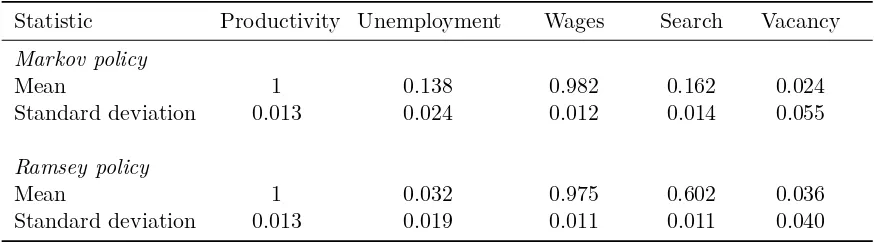
Table3compares steady states under the Ramsey and Markov policies. Not surprisingly, the Ramsey economy performs better than the Markov economy. The Markov government gives a much higher unemployment benefit than does the Ramsey government. The replacement ratio is 46% in the Markov economy, as opposed to 12% in the Ramsey economy. Although we do not calibrate to the Markov economy, its replacement ratio is much closer to the 40% replacement ratio as found in the U.S. economy. This suggests that non-commitment is a better description of the current U.S. policy. With higher benefit level, unemployed workers have less incentives to search. In fact, the Markov economy has much lower search intensity than the Ramsey economy.

Higher benefits give workers higher outside options, so wages are slightly higher in the Markov economy. Higher wages indicate lower profits for firms, and hence lower vacancy posting under the Markov policy. Lower search by workers and lower vacancy posting by firms lead to much higher unemployment level in the Markov economy. Therefore, output is lower and agents consume less in the Markov economy. In terms of welfare, the average consumption in the Markov economy has to increase by 4.84% to be equivalent to the Ramsey economy in steady state.

when the government lacks the ability to commit to future policies—as in the case of the Markov economy and almost all governments in reality—it cannot make any credible promise of lower benefit in the future. As a result, such government consistently provides higher than optimal benefits and leads the economy into a state of high unemployment, low output and low welfare.

5.2

Policy functions

In this section, we present and compare Ramsey and Markov equilibrium policy functions solved using cubic spline projection method.

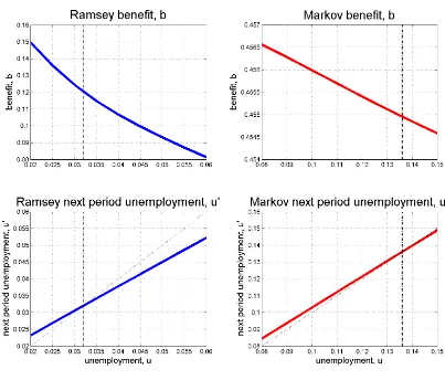
Figure 2 plots the Ramsey policy (left) and the Markov equilibrium policy (right) functions for benefit (top panels) and next period unemployment (bottom panels), holding productivity at the steady state level.22 _{In each plot, the solid line represent policy function, and the dashed line} indicates steady state unemployment rate.23

First, consider unemployment benefit (the top panels). The optimal unemployment benefit in the Ramsey case is decreasing in unemployment level, whereas the Markov benefit is only slightly decreasing in unemployment. One key difference between these two governments is that the Ramsey government internalizes the impact of its current policy on the actions of private sector in previous periods. When unemployment level is high, the marginal social benefit of job creation is higher, because the expected output gain of increasing vacancy positing is proportional to the number of unemployed workers. Thus the Ramsey government reduces unemployment benefit when unemploy-ment is high, in order to induce more search and vacancy posting in the previous period.

In contrast, the Markov government considers the previous period foregoneand hence does not internalize how previous period’s expectation of current policy impacts the economy in the past. But it still has some incentive to decrease benefits when unemployment is high, so as to encourage search in the current period. At the same time, as more workers are unemployed, the government, with a utilitarian objective function, has a stronger motive to provide insurance and help smooth consumption. Overall, these two effects almost cancel each other out, and the Markov government only slightly decreases benefits when unemployment is high.

The bottom panels of Figure2plot the next period unemployment policy functions𝑢′ associated with the Ramsey policy (left) and the Markov policy (right). In both cases, the policy function is increasing in current unemployment and coincides with the 45-degree line once at the steady state. Notice that the slope of the Ramsey unemployment is flatter than that of the Markov unemployment. This is because the Ramsey government, by planning a sequence of policies at time 0, has more control over the economy, and thus can move the next period unemployment further away from

22_{The Ramsey policy function plots also hold promised marginal utilitiesÛ}

⊗andÒ⊗at their respective steady state

level. Note that even though we solve Ramsey policies as functions, the solution to a Ramsey problem really should be understood assequences of variablesfrom𝑡=0 to𝑡=∞, given some initial state,(𝑢₀,𝑧₀)in this case.

Figure 2: Ramsey (left) and Markov (right) benefit (top panels) and unemployment (bottom panels) policy functions holding productivity at steady state. In each plot, the solid line denotes policy function, and the dashed line indicates steady-state unemployment level. The bottom panels als