Phase Field Simulation of the Effect of Elastic Inhomogeneity on Microstructure Evolution in Ni Based Superalloys

(1)

Phase-Field Simulation of the Eﬀect of Elastic Inhomogeneity

on Microstructure Evolution in Ni-Based Superalloys

Yuhki Tsukada

1;*

_{, Yoshinori Murata}

1

_{, Toshiyuki Koyama}

2

_{and Masahiko Morinaga}

1

Department of Materials, Physics and Energy Engineering, Graduate School of Engineering, Nagoya University, Nagoya 464-8603, Japan

2_{National Institute for Materials Science, Tsukuba 305-0047, Japan}

Phase-field simulation is performed to examine the effect of elastic inhomogeneity between the and0 _{phases on microstructure} evolution of the0_{phase in Ni-based superalloys. For solving the elastic equilibrium equation numerically in the elastically inhomogeneous} system, an iterative approach is used. In this simulation, both elastic anisotropy and shear modulus are varied independently based on the elastic constants of a practical Ni-based superalloy. Four different types of anti-phase domains in the0_{phase are also considered in this simulation. The} variation of elastic anisotropy affected significantly the manner of both morphology of the0_{phase and distribution function of the}0_particle size, whereas the variation of shear modulus did not affect them. [doi:10.2320/matertrans.MBW200826]

(Received October 20, 2008; Accepted February 10, 2009; Published March 25, 2009)

Keywords: phase-ﬁeld model, nickel-based alloys, elastic inhomogeneity

1. Introduction

Ni-based superalloys consisting of the 0 _{phase (L1}

2 structure) precipitated in thephase with face-centered cubic lattice are applied to gas turbine materials because of their excellent mechanical properties such as creep strength at high

temperatures. It is necessary to control the 0 _volume

fraction, morphology and size distribution of the (þ0₎ two-phase microstructure, since the mechanical properties of the superalloys are strongly related to them.

In recent years, the phase-ﬁeld model has been applied for simulating microstructure evolution in Ni-Al alloys.1–4)_The

phase-field model describes a microstructure using a set of conserved or non-conserved field variables. The micro-structure evolution can be simulated by a set of equations governing the evolution of the fields under the condition of achieving the minimum of the total free energy of the system. In previous works on Ni-based alloys,1,2,4) _{the difference}

in elastic constants between the and 0 _{phases (elastic} inhomogeneity) have not been considered in the calculation of the elastic strain energy, because the elastic inhomoge-neity is less than 7% in the wide range of temperatures in Ni-Al binary system.5) However, it is important to understand the eﬀect of the elastic inhomogeneity on the microstructure evolution, because the elastic inhomogeneity has become about 13% in a practical Ni-based superalloy at high temperatures.6)

There are some models considering the elastic

inhomoge-neity in the phase-ﬁeld model.7,8) _{For example, Hu and}

Chen8) _{proposed a very eﬃcient phase-ﬁeld model for}

elastically inhomogeneous systems, in which an iterative approach is used for solving the elastic equilibrium equation numerically. They concluded that it required a rather strong elastic inhomogeneity (>50%) to produce precipitate mor-phology diﬀerent dramatically from one obtained in elasti-cally homogeneous systems. However, the eﬀect of the elastic inhomogeneity in Ni-based alloys should be assessed in the condition taking into account the four types of

anti-phase domains existing in the0_{phase, because Wang}_{et al.}1)

reported that the ordered nature of the precipitate played an important role in the microstructure evolution.

The purpose of this study is to examine the effect of the elastic inhomogeneity on microstructure evolution of the0 phase in Ni-based superalloys by the phase-field simulation. In the elastic energy calculation, the elastic constants are based on a practical alloy and the iterative approach is used for solving the local displacement vector. Four different types of anti-phase domains in the0phase are also considered in this simulation.

2. Calculation Model

In order to simulate microstructure change of theand0 phases, the volume fraction of the0 _phase _f_ð_r_;_t_Þ_{and four} artificial order parameters iðr;tÞði¼1;2;3;4Þ, which de-scribe the four different domains in the L12 phase structure, are chosen as field variables. These field variables vary spatially (r) and temporally (t). Usually, alloy composition cðr;tÞis used as a field variable,1–4)butfðr;tÞis used instead ofcðr;tÞin this study, because fðr;tÞis suitable to treat the multi-component systems when the phase-field model is applied to the practical Ni-based alloys. The temporal evolution of the field variables is given by solving the following Cahn-Hilliard and Ginzburg-Landau equations:

@fðr;tÞ @t ¼Mr

2 Gsys

fðr;tÞ; ð1Þ

@iðr;tÞ

@t ¼ L

Gsys

iðr;tÞ

ði¼1;2;3;4Þ; ð2Þ

whereGsys is the total free energy of the system,M is the

diﬀusion mobility and L is the structural relaxation coef-ﬁcient. The total free energy of the system is given by,

Gsys¼

Z

r

½Gchemðf; iÞ þEgradðiÞ þEstrðiÞdr; ð3Þ

whereGchemis the chemical free energy density,Egradis the

gradient energy density and Estr is the elastic strain energy

density. The chemical free energy density is expressed as, *_{Graduate Student, Nagoya University}

(2)

Gchem¼ f1hðiÞgGmchemðfmÞ

þhðiÞGp_chemðfpÞ þwgðiÞ; ð4Þ

wherewis the double-well potential height.3,4)_{In this study,}

the chemical free energy density of the matrix and the0 precipitate,Gm

chemandG p

chem, are given as,

Gm_chem¼1

2W1f 2

; ð5Þ

Gp_chem¼1

2W2ð1fÞ

2_; _ð6Þ

where W1 and W2 are the coeﬃcients determined by the

Gibbs energy calculation based on the sub-lattice model using the thermodynamic database. The functions hðiÞand gðiÞare selected as,

hðiÞ ¼

X4

i¼1

½3_ið1015iþ62iÞ; ð7Þ

gðiÞ ¼

X4

i¼1

½2_ið1iÞ2 þ

X4

i¼1 X4

j6¼i

2_i2_j: ð8Þ

Employing the description proposed by Kim et al.,9) _the

interface region is regarded as a mixture of the and 0 phases with diﬀerent volume fractions of the 0 _{phase but} with equal chemical potentials:

f ¼ f1hðiÞgfmþhðiÞfp

@Gm_chem

@f

f¼fm ¼ @G

p chem

@f

f¼fp

: ð9Þ

The gradient energy density is estimated from the artiﬁcial order parameters as,

Egrad¼

1

2 X4

i¼1

ðriÞ2; ð10Þ

where is the gradient energy coeﬃcient of the order

parameter.10)_{The elastic strain energy density arising from}

the lattice misﬁt between the and 0 _{phases is estimated} based on the micromechanics:11,12)

Estr¼

1 2Cijkl"

el ijðr;tÞ"

el

klðr;tÞ: ð11Þ

The elastic strain,"el_kl, is expressed as,

"el_klðr;tÞ ¼"c_klðr;tÞ "0_klðr;tÞ; ð12Þ

where "c

kl and "0kl represent the constrained strain and

eigenstrain, respectively. The eigenstrain is expressed as,

"0_klðr;tÞ ¼"0klfhðiÞ hðiÞg; ð13Þ

and

"0 ¼amap

am

; ð14Þ

where"0represents the lattice misﬁt andklis the Kronecker

delta function. In eq. (14), am and ap are the lattice

parameters of the matrix and the 0 _precipitate, respec-tively. In eq. (12), the constrained strain can be expressed as,

"c_klðrÞ ¼1 2

@ukðrÞ

@rl þ

@ulðrÞ

@rk

; ð15Þ

whereurepresents the local displacement vector.

The Hooke’s law gives the local elastic stress as el

ijðrÞ ¼Cijkl"elklðrÞ, and the local elastic constants Cijkl is

assumed to beCijkl¼ f1hðiÞgCmijklþhðiÞC

p

ijklin eq. (11),

whereCm

ijkl andC

p

ijkl represent the elastic constants of the

matrix and the 0 _{precipitate, respectively. From the local} mechanical equilibrium equation, i.e.,@el

ij=@rj¼0, the local displacement vector in eq. (15) is solved in Fourier space by applying the iterative approach.8)_{The number of iterations}

depends on the degree of the elastic inhomogeneity.

3. Results

Phase-ﬁeld simulation at a temperature of 1373 K was performed by solving the two sets of eqs. (1) and (2) numerically, using the explicit method under the periodic boundary conditions. The coeﬃcients of the chemical free energy density in eqs. (5) and (6) were determined asW1¼ 1:20103 _and _W

2¼1:45103Jmol1 based on the

Gibbs energy calculation using the thermodynamic data-base.13) _{By ﬁtting to the interfacial energy density, which}

has the value of 14.2 mJm2 _{in Ni-Al binary alloys,}14)_the

double-well potential height and the gradient energy coef-ﬁcient were determined as w¼1:7107_J_m3 _and

¼

2:11010_J_m1_{, respectively. Elastic constants of the}

TMS-26 alloy at 1373 K (Cm

11¼184, C12m ¼135, Cm44¼ 88:1, C₁₁p ¼209, C₁₂p ¼142, C₄₄p ¼90:4GPa)6) were em-ployed in this simulation, and the volume fraction of the0 phase in the equilibrium state was set to be 55%.6)The lattice misfit was set to be"0¼ 0:003, which is close to the value for TMS-26 alloy.6)Except for the elastic constants, physical constants for Ni-Al binary system were employed in this study, because the focus of this study is to examine the effect of the elastic inhomogeneity on the microstructure evolution qualitatively. The simulation was started from the super-saturated solid solution with a random noise of the field variables (f; i).

3.1 Morphology

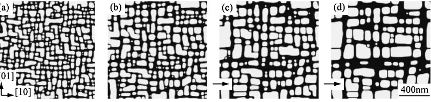
Figure 1 shows 2D morphological evolution of the 0

phase in the late stage of coarsening at 1373 K calculated from the phase-ﬁeld simulation using the elastic constants of the TMS-26 alloy. The0_{phase is expressed as white area in} Fig. 1. The cuboidal shape of the0phase arranged along the h10i crystallographic direction of the matrix is observed due to the anisotropic elastic interaction. Furthermore, the coalescence of the neighboring0_{phases with the same order} parameter is observed as marked by arrows in Figs. 1(c) and (d), the coalescence of which has been also reported from the simulation in Ni-Al alloys.4)

(3)

ðBm_;_Bp_{Þ ¼ ð319;}_351Þ_,_ð_Gm_;_Gp_{Þ ¼ ð176;}_180Þ_and_ðm_;p_{Þ ¼}

ð3:59;2:69Þ. Here, the superscripts m and p represent the elastic constants of the and0_{phases, respectively.}

Figure 2 shows the results of the phase-ﬁeld simulation obtained in the late stage of coarsening of the 0 _phase,

indicating the dependence of the 0 _{morphology on the}

anisotropy in theand0_{phases. The anisotropy is varied in} ﬁve sets asðm; pÞ ¼ ð6:07;2:17Þ, (4.51, 2.40), (3.59, 2.69), (2.98, 3.07), (2.55, 3.57). In this simulation, both bulk and shear modulus are kept to be constant. It is observed in Fig. 2 that the cuboidal0_{phase shows irregularity when the ratio of} p _to m _{becomes large (see Fig. 2(e)). Figure 3 shows the}

simulation results obtained in the late stage of coarsening of the0_{phase, indicating the dependence of the}0_morphology

on the shear modulus in the and 0 _{phases. The shear}

modulus is varied in ﬁve sets as (¼Cp₄₄=Cm

44¼0:90, 1.02, 1.16, 1.32, 1.74). In this simulation, both bulk modulus and anisotropy are kept to be constant. It is found that the elastic inhomogeneity caused by the diﬀerent ratios of the shear

modulus in the and 0 _{phases aﬀects scarcely the}

morphology of the0_phase.

3.2 Particle size distribution

From the simulation results, scaled particle size distribu-tion of the0 _{phase was obtained by measuring the fraction}

of the0 _{particles having a radius (}_r_{) within a size interval} which was normalized by the average radius (r). The particle size distribution is obtained from the result for each time step. In this study, according to a similar way to Vaithyanathan and Chen,2) _{averaged particle size distribution was}

con-structed from the results for four different time steps corre-sponding to Fig. 1. Figure 4 shows the scaled particle size distributions obtained from simulation results for five differ-ent conditions corresponding to Fig. 2, in which the aniso-tropy in the and0phases are changed independently. It is shown that the spectrum becomes broad with increasing the ratio ofp_tom_{, while the radius showing the maximum size}

distribution (hereafter called as peak radius) does not change and it is almost at 0.75 in the normalized radius. Figure 5 shows the scaled particle size distributions obtained from simulation results for five different conditions corresponding to Fig. 3, in which only the ratio of the shear modulus in the and0_{phases is changed independently. From Fig. 5,} it is found that both the peak radius and the spectrum shape are not affected by the variation of the shear modulus.

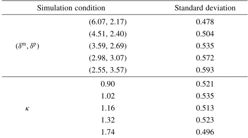
The eﬀect of the elastic inhomogeneity on the standard deviation of the particle size distribution is summarized in Table 1. It is obvious that the variation of the anisotropy broadens the spectrum of particle size distribution but that the variation of the shear modulus does not aﬀect it.

Fig. 1 Morphological evolution of the0_{phase calculated from 2D phase-ﬁeld simulation at 1373 K using the elastic constants of a} practical Ni-based superalloy. (a)t¼10000, (b)t¼20000, (c)t¼40000and (d)t¼80000. All time expressed here are dimensionless time steps.

Fig. 2 Dependence of the0_{phase morphology on elastic anisotropy in the}_{matrix and}0_{precipitate. (}m_;p_{): (a) (6.07, 2.17), (b) (4.51,}

2.40), (c) (3.59, 2.69), (d) (2.98, 3.07) and (e) (2.55, 3.57).is2C44=ðC11C12Þ.

Fig. 3 Dependence of the0 _{phase morphology on shear modulus in the} _{matrix and}0_{precipitate. (a)}_¼₀_:₉₀_{, (b)}_¼₁_:₀₂_{, (c)} ¼1:16, (d)¼1:32and (e)¼1:74.isCp₄₄=Cm

[image:3.595.89.510.72.172.2] [image:3.595.86.514.224.314.2] [image:3.595.84.513.356.446.2]

(4)

4. Discussion

From the phase-ﬁeld simulation based on the variation of only the anisotropy in the and0 _{phases, it is found that}

the 0 _{phase shows unstable shape as shown in Fig. 2(e)}

when the ratio of p _tom _{becomes large. In the previous}

work, Hu and Chen8)_{showed that elastic energy became low}

when hard precipitates were surrounded by soft matrix comparing to that soft precipitates were surrounded by hard matrix. The simulation condition of Fig. 2(e) is the case that the Young’s modulus of the 0 _{phase is just slightly} larger than that of the phase. This condition seems to be

the reason why the cuboidal 0 phase became unstable in

Fig. 2(e).

Furthermore, the variation of the anisotropy aﬀected the particle size distribution as shown in Fig. 4 and Table 1. Vaithyanathan and Chen2) _{studied the eﬀect of precipitate}

volume fraction on the particle size distribution and showed that the increase in volume fraction of the 0 _{phase shifts} the peak radius to smaller normalized radius and leads to broadening of the distribution. In the particle size distribu-tions obtained in this study, the peak radius is similar, i.e., r=rrðtÞ ¼0:70:8(see Figs. 4 and 5), which is consistent with the position reported by Vaithyanathan and Chen,2)_{when the}

volume fraction of the precipitate is about 55%. It is interesting that the variation of the anisotropy aﬀected only width of the distribution spectrum without changing the peak radius as shown in Table 1. It should be emphasized that the diﬀerence of about 20% in elastic constants between the

and 0 _{phases aﬀected both precipitate morphology and}

particle size distribution (see Figs. 2 and 4).

The eﬀect of the diﬀerence in the shear modulus between the matrix and the precipitate has been also reported previously,7,8)_{but it was examined based on the same elastic}

constants for both the matrix and the precipitate. In this study, however, the elastic constants for each phase are based on the practical ones for TMS-26, and the variation of the shear modulus did not aﬀect both morphology and particle size distribution of the 0 _{phase. This is probably because the} anisotropy in the two phases aﬀected mainly the stability of the 0 _{morphology. In other words, under the conditions of} the variation of the shear modulus employing in this study,

the cuboidal 0 phase was stable by the eﬀect of the

anisotropy in the and0_phases.

Fig. 4 Scaled particle size distributions obtained from simulation results for ﬁve diﬀerent conditions corresponding to Fig. 2, varying only elastic anisotropy in thematrix and0_{precipitate. (}m_;p_{): (a) (6.07, 2.17), (b) (4.51, 2.40), (c) (3.59, 2.69), (d) (2.98, 3.07) and}

(e) (2.55, 3.57). In all cases, averaged results are shown which are obtained from simulation results for four diﬀerent time steps corresponding to Fig. 1.

[image:4.595.92.511.71.176.2]

Fig. 5 Scaled particle size distributions obtained from simulation results for five different conditions corresponding to Fig. 3, varying only shear modulus in thematrix and0_{precipitate. (a)}_¼₀_:₉₀_{, (b)}_¼₁_:₀₂_{, (c)}_¼₁_:₁₆_{, (d)}_¼₁_:₃₂_{and (e)}_¼₁_:₇₄_{. In all cases,} averaged results are shown which are obtained from simulation results for four different time steps corresponding to Fig. 1.

Table 1 Standard deviation of size distribution curves of the0_particles obtained from diﬀerent simulation results as shown in Figs. 4 and 5.

Simulation condition Standard deviation

(6.07, 2.17) 0.478 (4.51, 2.40) 0.504 (m_;p₎ _{(3.59, 2.69)} _0.535

(2.98, 3.07) 0.572 (2.55, 3.57) 0.593

0.90 0.521

1.02 0.535

1.16 0.513

1.32 0.523

[image:4.595.93.511.255.360.2] [image:4.595.45.291.455.592.2]

(5)

It is known that the elastic interactions aﬀect the shape of the particle size distribution.2) _{However, as long as we}

know, this is the ﬁrst simulation showing that the elastic inhomogeneity aﬀects the width of the size distribution spectrum.

5. Conclusions

2D phase-field simulation was carried out to examine the effect of elastic inhomogeneity on the microstructure evolution in Ni-based superalloys. Based on the elastic constants of a Ni-based superalloy, both anisotropy and shear modulus in the and0 _{phases were varied independently.} The variation of the anisotropy affected the morphology of the 0 phase and caused the cuboidal shape unstable when the ratio of p to m was large. Furthermore, the variation of the anisotropy affected only width of the distribution spectrum of the 0 _{particle size without changing the peak} radius. On the other hand, the variation of the shear modulus did not affect both morphology and particle size distribution of the0 _phase.

REFERENCES

1) Y. Wang, D. Banerjee, C. C. Su and A. G. Khachaturyan: Acta Mater.

46(1998) 2983–3001.

2) V. Vaithyanathan and L. Q. Chen: Acta Mater.50(2002) 4061–4073. 3) J. Z. Zhu, T. Wang, S. H. Zhou, Z. K. Liu and L. Q. Chen: Acta Mater.

52(2004) 833–840.

4) J. Z. Zhu, T. Wang, A. J. Ardell, S. H. Zhou, Z. K. Liu and L. Q. Chen: Acta Mater.52(2004) 2837–2845.

5) S. V. Prikhodko, J. D. Carnes, D. G. Isaak, H. Yang and A. J. Ardell: Metall. Mater. Tran. A30(1999) 2403–2408.

6) K. Tanaka, T. Kajikawa, T. Ichitsubo, M. Osawa, T. Yokokawa and H. Harada: Mater. Sci. Forum475–479(2005) 619–622.

7) P. H. Leo, J. S. Lowengrub and H. J. Jou: Acta Mater.46(1998) 2113– 2130.

8) S. Y. Hu and L. Q. Chen: Acta Mater.49(2001) 1879–1890. 9) S. G. Kim, W. T. Kim and T. Suzuki: Phys. Rev. E60(1999) 7186–

7197.

10) J. W. Cahn and J. E. Hilliard: J. Chem. Phys.28(1958) 258–267. 11) A. G. Khachaturyan:Theory of structural transformations in solids,

(Wiley, New York, 1983).

12) T. Mura: Micromechanics of Defects in Solids, 2nd revised ed., (Kluwer Academic, 1991).

13) I. Ansara, N. Dupin, H. L. Lukas and B. Sundman: J. Alloy. Compd.

247(1997) 20–30.