The impact of body weight on occupational mobility and career development

Munich Personal RePEc Archive

The impact of body weight on

occupational mobility and career

development

Harris, Matthew

University of Tennessee

28 January 2015

The Impact of Body Weight on Occupational Mobility

and Career Development

Matt Harris

University of Tennessee

January 28, 2015

Abstract

This paper examines the relationship between individuals’ weight and their employ-ment decisions over the life cycle. I estimate a dynamic stochastic model of individuals’ annual joint decisions of occupation, hours worked, and schooling. The model allows body weight to affect non-monetary costs, switching costs, and distribution of wages for each occupation; and also allows individuals’ employment decisions to affect body weight. I use conditional density estimation to formulate the distributions of wages and body weight evolution. I find that heavier individuals face higher switching costs when transitioning into white collar occupations, earn lower returns to experience in white-collar occupations, and earn lower wages in socially intensive jobs. Simulating the model with estimated parameters, decreased occupational mobility accounts for 10 percent of the obesity wage gap. While contemporaneous wage penalties for body weight are small, the cost over the life cycle is substantial. An exogenous increase in ini-tial body mass by 20 percent leads to a 10 percent decrease in wages over the life course.

Keywords: Labor, occupational choice, obesity, dynamic discrete choice, productivity, switching costs

∗_{I would like to thank Donna Gilleskie, Brian McManus, David Guilkey, Helen Tauchen, Clement Joubert,}

Maarten Lindeboom, William Neilson, and participants in the UNC Applied Microeconomics Workshop, Triangle Health Economics Workshop, and 6th Biennial Conference of the American Society of Health Economists.

†_{Department of Economics and Center for Business and Economic Research, 722 Stokely Management}

1

Introduction

How does body weight affect employment behavior and wages over the life cycle? We

know obesity yields high costs in the workplace.1 _{In addition to the oft cited health care}

costs, estimates place annual workplace productivity costs of obesity between $12 and $30

billion. While obese workers miss 15 to 50 percent more work time than the healthy weight,

two-thirds of these productivity costs are due to decreased at-work performance. Reduced

productivity not only affects contemporaneous wages and employment decisions, but also

decreases subsequent pay increases and employment opportunities (Holmstrom, 1999). Body

weight today therefore affects expected future wages and labor market opportunities.

The workplace costs of high body weight are inherently dynamic and vary by

occu-pation. Studies have shown obesity leads to difficulty managing professional interpersonal

relationships and reduces stamina when performing physical tasks.2 _{While lower productivity}

affects wages, difficulties with certain job requirements may yield additional non-monetary

costs and therefore influence occupational choices. An individual’s body weight may also

provide a signal about that individual’s self-discipline or work ethic, the value of which may

differ between occupations. Such a negative signal would lead to decreased occupational

mobility for individuals of higher body weight.3 _{Occupational differences in the costs of high}

body weight provide additional motivation for modeling these costs as a part of

forward-looking individuals’ employment decisions. When an individual chooses an occupation, he

accrues human capital that is not perfectly transferable to other occupations (Kambourov

and Manovskii, 2009). Thus, contemporaneous occupational choice affects both expected

future wages and future occupational decisions. Finally, an individual’s body weight is itself

dynamic, and maybe affected by one’s choice of occupation and hours.

1

See, for example Ricci and Chee (2005), and Andryeva (2014)

2

See Pronk et al. (2004); Johar and Katayama (2012); Hamermesh and Biddle (1994); DeBeaumont (2009); Han et al. (2009)

3

Despite the inherent dynamic relationship between body weight and employment

out-comes, the existing literature on the subject has largely relied on static approaches and

abstracted from either occupational choice or wages.4 _{I formulate and estimate a dynamic}

discrete choice model where body weight affects both the distribution of wage offers and

non-monetary costs of each employment alternative; and employment decisions subsequently

affect weight.5 _{Both the model and method follow in the dynamic discrete occupational}

choice literature (Keane and Wolpin, 1997; Altug and Miller, 1998; Lee, 2005; Lee and

Wolpin, 2006; Flabbi, 2010; Sullivan, 2010; Gayle and Golan, 2012; Eckstein and Lifshitz,

2011; Yamaguchi, 2013; Baird, 2014). I construct indices of the intensity of mental,

phys-ical and social job requirements for each occupation to determine how the monetary and

non-monetary costs of body weight in the workplace vary with these requirements.

I estimate the parameters governing the individuals’ decision making process using

data from the National Longitudinal Survey of Youth, 1979 cohort. The model is solved in a

finite-horizon setting, using backwards recursion, value function interpolation and maximum

likelihood estimation (Keane and Wolpin, 1994; Mroz and Weir, 2003). Consistent with

earlier work, I do not find large, direct wage contemporaneous penalties for high body weight

(Cawley, 2004). I do find that high body weight presents significant barriers to occupational

mobility and inhibits career development over the life cycle. Results indicate that one weight

class (35 pounds on a 6-foot male), leads to an additional $6,500 in switching costs when

transitioning into professional and managerial occupations. These switching costs account

for 25 percent of the occupational attainment gap between obese and non-obese workers. By

affecting early career occupational choices, these costs lead to differences in human capital

and subsequent wages. High body weight impedes career development in other ways as well.

Individuals of high body weight are also found to earn lower returns to experience in white

4

Section2reviews papers that examine body weight and wages, or occupational choice and body weight, or occupational choice and wages.

5

collar occupations, and face lower wages and higher non-monetary costs in socially intensive

jobs. The non-monetary costs (including switching costs) of employment are not recoverable

without modeling the individual’s forward looking employment decision.

I use semi-parametric methods to estimate the full distribution of wages (conditional on

body weight, experience, education, job requirements, etc.) inside the model. Individuals of

high body weight are much less likely to be observed in the upper quantiles of the distribution

of wages. All wage differentials for high body weight, including lower returns to white-collar

experience, education, and lower wages in socially intensive jobs, stem from the reduced

probability of receiving wage offers from the upper quartile of the wage distribution. The

combination of these results indicates that body weight is a significant impediment to career

progress in white collar occupations.

Using the estimated parameters of the model, I simulate the dynamic effects of a

con-siderable (5 BMI points) exogenous weight reduction on a 35 year-old individual. While

instantaneous effects are small (wages increase by 4 percent) the dynamic effects are

sub-stantial. Relative to the baseline, the 45 year old individual who experienced an exogenous

shock at age 35 is nearly 5 percent more likely to be in a managerial occupation, 10

per-cent more likely to attain work in a sales or administrative occupation, and the individual’s

overall expected wage increases by 10 percent.

In summary, I find that while contemporaneous aggregate wage penalties for body

weight are small, that high body weight nevertheless presents significant costs to

work-ers. Over the life cycle, high body weight decreases occupational mobility, decreases wages,

increases non-monetary costs in socially intensive jobs, and particularly decreases the

prob-ability of receiving wage offers in the upper quantiles of the distribution of wages.

This paper proceeds as follows. Section2 provides a brief motivation and background

on the relationships between body weight and employment outcomes. Section 3 describes

the relevant data: the National Longitudinal Study of Youth, 1979 cohort, the Dictionary of

the dynamic model. Section 5 discusses identification and the empirical implementation

of the theoretical model. Section 6 contains the parameter results and discusses how the

model predicts the variation of interest in the data. Section 7 contains the counterfactual

simulations using the estimated parameters of the model, and Section 8 concludes with a

brief discussion.

2

Relevant Literature

This paper contributes to a few different subsets of the literature. Specifically, I

con-tribute to the literature on dynamic models of forward looking individuals’ occupational

decisions as cited above. Within that literature, this is first paper to examine differences

in earnings and occupational attainment on the basis of body weight in a dynamic

dis-crete occupational choice framework. In so doing, this paper extends the literature on body

weight and labor market outcomes. Most prior work in that literature has focused on the

effects of individuals’ weights on their wages, utilized static methods, and abstracted from

modeling occupational choice (Cawley, 2004; Pagan and Davila, 1997; Johar and Katayama,

2012; Hamermesh and Biddle, 1994; Han et al., 2009).6 _{Dynamic models of differences in}

occupational choice and wage differences have more often been utilized in examining the

gender wage gap (e.g., Altug and Miller (1998); Gayle and Golan (2012); Eckstein and

Lif-shitz (2011); Flabbi (2010); Yamaguchi (2013)) and black-white wage gap (e.g., Keane and

Wolpin (2000); Bowlus and Eckstein (2002); Lehmann (2013)).

This paper also contributes to a growing literature where job requirements are

in-corporated into dynamic models as a determinant of occupational choice (Sanders, 2010;

Yamaguchi, 2012). In permitting contemporaneous employment decisions to affect future

body weight, I also contribute to the literature on how one’s employment behavior affects

6

one’s health (King et al., 2001; Lakdawalla and Philipson, 2002; Kelly et al., 2011;

Courte-manche, 2009; Ravesteijn et al., 2014).

Additionally, this paper incorporates prospective wage differentials into a single-agent

occupational choice framework. Theoretically, the model seeks to merge Mincer (1958),

Ben-Porath (1967), and Becker (1957). Prior dynamic models in this area have have typically

used a general equilibrium approach and focused on search rather than occupational choice

to better identify discrimination. The structure of this model closely resembles Keane and

Wolpin (1997) and Sullivan (2010), focusing on how current and expected future monetary

and non-monetary costs affects individuals’ decisions over the life cycle. As Coate and Loury

(1993) show, anticipated wage differentials can affect the formation of human capital, which

affects subsequent wages. In this model, weight-related wage differentials are incorporated

into the individual’s dynamic optimization problem. Forward-looking agents choose

occupa-tions and amount of labor to supply mindful of expected future wages, returns to experience,

and switching costs, all of which vary by body weight.

There is also a small methodological contribution to the literature on dynamic models of

occupational choice regarding the distribution of unobserved wages. Often when integrating

over missing prices or wages, parametric distributions are assumed as in Stinebrickner (2001).

Here, I estimate the full distribution of wages inside the model using conditional density

estimation (Gilleskie and Mroz, 2004). When integrating over missing wages, I can use the

full estimated density of those unobserved wages when performing quadrature to calculate

choice probabilities.

3

Data

The data come from three sources. The data on individuals’ wages, employment

Survey of Youth, 1979 cohort (NLSY ’79). Data on job requirements comes from the

Dictio-nary of Occupational Titles (DOT) and its successor, the Occupational Information Network

(O*NET). City level data on food prices come from the 4th quarter reports from ACCRA

(formerly the Inter-City Cost of Living Index).

The NLSY ’79, conducted by the Bureau of Labor Statistics, follows a nationally

rep-resentative cohort of youths initially aged 14-22 annually from 1979 to 1994 and biennially

to 2010.7 _{Respondents were asked questions regarding family background, schooling,}

occu-pation, hours of work, wages, criminal activity, health, etc. Weight data are recorded for

1981, 1982, and in each wave since 1985. The NLSY ’79 is the longest running nationally

representative panel that contains data on weight, wages, and employment decisions. The

estimation sample is restricted to white males. Individuals that missed an interview in the

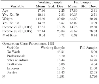
biennial phase were dropped. 8 _{Table 1 details the sample construction. The final sample}

consists of 29,693 person-year observations. Descriptive statistics for the full sample of white

males and the estimation sample are available in Table 2.

Table 1: Sample Construction N Description

12,686 National Longitudinal Survey of Youth, 1979 cohort, full sample 3,720 Sample after restricting demographics to white males

2,566 Sample after dropping poor white and military oversample

1,291 Sample after dropping those individuals missing an interview in the biennial phase

1291 unique individuals yields 29,693 person/year observations

Source: _{National Longitudinal Survey of Youth, 1979 cohort}

Individuals’ reported occupations are classified as one of five major categories from the

1970 Census Occupational Classification System.9 _{Table3lists the five occupation categories}

7

http:\\www.nlsinfo.org

8

I restrict the sample to white males to keep an already heavily parameterized model computationally feasible. Including females and other races would involve cultural norms, require parameters for demographic shifters on all variables of interest. Similarly, keeping individuals who miss interviews during the biennial phase would involve integrating over missing histories, choices and state variables during those years, creating substantial additional computational difficulties.

9

Table 2: Summary Statistics- Full v. Working Sample of 1979 NLSY Working Sample Full Sample Variable Mean Std. Dev. Mean Std. Dev.

Age 17.36 2.25 17.89 2.31

Yrs. Ed.’79 10.41 2.83 10.33 2.71

Weight 144.50 29.69 145.50 29.70

Yrs. Ed ’98 13.52 5.57 13.02 4.99

Income 79 ($1,000’s) 17.81 13.18 14.78 12.50 Income 98 ($1,000’s) 27.14 26.84 25.52 26.53

# of Kids 0.34 0.71 0.37 0.74

Occupation Class Percentages, 1981

Variable Working Sample Full Sample

No Work 46.51 5.09

Professionals 5.70 5.31

Sales & Admin 16.44 14.76

Craftsmen 5.08 4.84

Laborers 13.15 11.60

Service 14.43 12.35

N 1,291 3,720

used in this research and displays the proportion of obese and non-obese individuals selecting

into these occupations for three time periods.

3.1

Preliminary Evidence on Weight, Wages, and Employment

Behavior

Preliminary examination of the data yields evidence of differences in optimal

employ-ment behavior and wages related to body mass. While this study treats body mass as a

continuous variable both theoretically and empirically, the following statistical analyses use

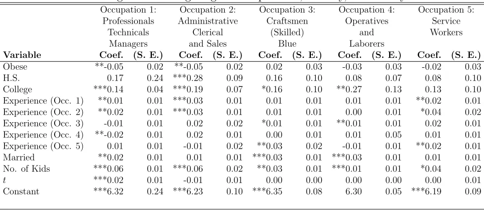
an indicator function for whether the individual is obese.10 _{Table 4 contains the results of}

fixed effects regressions of log wages on a dummy variable for whether the individual is obese,

years of experience in each of the five occupational categories, indicators for if the individual

has graduated high school and college, family state, and a time trend. The results indicate

10

The Centers for Disease Control define obesity as a Body Mass Index (kg/m2

Table 3: Occupational Sorting - Proportions of Obese and Non-Obese Workers by Occupation Category

Occupation 1: Occupation 2: Occupation 3: Occupation 4: Occupation 5: Professionals Administrative Craftsmen Operatives Service

Technicals Clerical (Skilled) and Workers Managers and Sales Blue Laborers

Ages Bt<30 Bt≥30 Bt<30 Bt≥30 Bt<30 Bt≥30 Bt<30 Bt≥30 Bt<30 Bt≥30 24-30 24.80 15.51 11.96 9.74 17.80 22.07 21.8 28.83 8.28 10.93

31-37 36.33 27.24 12.25 12.23 19.52 24.59 20.36 21.82 6.31 9.71

38-45 40.51 37.17 9.25 9.99 18.25 19.77 15.47 15.31 6.52 7.91

Table 4: Fixed Effect Regression of Log Wages on Experience, Obesity, and Family Variables

Occupation 1: Occupation 2: Occupation 3: Occupation 4: Occupation 5: Professionals Administrative Craftsmen Operatives Service

Technicals Clerical (Skilled) and Workers Managers and Sales Blue Laborers

Variable Coef. (S. E.) Coef. (S. E.) Coef. (S. E.) Coef. (S. E.) Coef. (S. E.)

Obese **-0.05 0.02 **-0.05 0.02 0.02 0.03 -0.03 0.03 -0.02 0.03 H.S. 0.17 0.24 ***0.28 0.09 0.16 0.10 0.08 0.07 0.08 0.10 College ***0.14 0.04 ***0.19 0.07 *0.16 0.10 **0.27 0.13 0.13 0.10 Experience (Occ. 1) **0.01 0.01 ***0.03 0.01 0.01 0.01 0.01 0.01 **0.02 0.01 Experience (Occ. 2) **0.02 0.01 ***0.03 0.01 0.01 0.01 0.00 0.01 *0.04 0.02 Experience (Occ. 3) -0.01 0.01 0.02 0.02 *0.01 0.01 **0.01 0.01 0.02 0.01 Experience (Occ. 4) **-0.02 0.01 0.02 0.01 0.00 0.01 0.01 0.05 0.01 0.01 Experience (Occ. 5) 0.01 0.01 -0.01 0.02 **0.03 0.02 -0.01 0.01 **0.02 0.01 Married **0.02 0.01 0.01 0.01 ***0.03 0.01 ***0.03 0.01 0.01 0.01 No. of Kids ***0.06 0.01 ***0.06 0.02 **0.03 0.01 ***0.01 0.01 *0.04 0.02

t ***0.02 0.01 -0.01 0.01 0.00 0.00 0.00 0.00 0.00 0.01 Constant ***6.32 0.24 ***6.23 0.10 ***6.35 0.08 6.30 0.05 ***6.19 0.09

that obese individuals face lower wages, but these differences are statistically significant only

in ‘white-collar’ occupations. Additionally, returns to own and cross-occupational experience

vary by occupation. Experience in the five categories is not rewarded equally.

The data also show that individuals of high body mass exhibit differences in

occupa-tional choice frequencies that create subsequent differences in human capital. Figure2shows

that obese individuals are less likely to work in white collar occupations than the non-obese,

particularly early in their careers. Note the white collar occupations are also the ones that

exhibit negative wage differentials for body weight. It is unclear whether these differences

induce the observed differences in employment behavior. Another implication of these

by weight in earlier periods. Because experience affects future wages, understanding the

re-lationship between body mass and wages requires understanding how body mass influences

optimal employment behavior. From the regression and bar chart, note the obese sort into

the occupations that yield less valuable experience. Experience in blue collar and service

jobs is minimally valued in white collar occupations. The obese and non-obese also differ in

their occupational transition patterns. Table10(see Section6) summarizes these differences.

Figure 3 depicts the difference in average real wages between obese and non-obese

workers for each of the five occupational categories for each age in the sample period. The

obese earn equal or lower wages than the non-obese in all categories. The differential in real

wages for white collar occupations quadruples over the sample period: obese workers earn

approximately one dollar per hour less than their non-obese counterparts at age 25, but four

dollars less at age 49.11

3.2

Dictionary of Occupational Titles and Occupational

Informa-tion Network

The data used to construct indices of job requirements come from the DOT and

O*NET. The data on job requirements are taken from the 1977 edition, 1982 updates, 1986

updates, and 1991 revision. In the mid-1990s, the DOT was deemed obsolete and replaced

with the O*NET, the first release of which was in 1998. In contrast to the DOT, the O*NET

is aligned with the Census system of occupation classification and provides information on

between 850-1000 ‘job families’. The O*NET focuses on white-collar occupations and on

information and service jobs, and it contains much finer numerical ratings (on level and

im-portance) for far more requirements per occupation. AppendixB contains additional details

on forming the requirement indices.

11

3.3

ACCRA Data on Food Prices

Food price ratios were constructed using data from C2ER.12 _{The data contain prices of}

commonly purchased items as reported by Chambers of Commerce in over 200 Metropolitan

Statistical Areas, including: T-bone steaks, ground hamburger, iceberg lettuce, tomatoes,

canned green beans, 2-piece fried chicken meals, McDonalds quarter-pounders, and Pizza

Hut/Pizza Inn 12-inch pizzas. I utilize annual data from 1976 to 2008 to construct a

fast-food-to-produce price index. These local indices are then linked to the Geocoded NLSY data.

These indices proxy for the costs of consuming healthy food relative to unhealthy food over

the sample period.13 _{Additional data on construction of food price ratios and geographic}

matching is available in AppendixB.

4

Dynamic Stochastic Discrete Choice Model

I specify a dynamic stochastic model of employment behavior in which body weight

and the requirements of the job affect both the distribution of wages and non-monetary costs

of each alternative. Subsection 4.1 defines the set of alternatives. Subsections 4.2 and 4.3

define the components of contemporaneous utility from each alternative. Subsections 4.4

and 4.4.1 discusses the distribution of wages and growth of human capital. Subsection 4.5

discusses the weight transition equation and Subsection 4.6 assembles these components to

formulate the individual’s dynamic optimization problem in a value function framework.

4.1

Set of Alternatives

In this model agents jointly decide whether to work, how much to work, in which

occupation to work, and whether to attend school. There are a total of 23 alternatives,

12

Formerly ACCRA and The Inter-City Cost of Living Index

13

hj ∈ HJ, available to an individual in each discrete period. The employment alternatives,

h, are:

h= 1 : work part time: weekly hours ∈ {15,34}

h= 2 : work full time: weekly hours∈ {35,49}

h= 3 : work more-than-full-time: weekly hours≥ 50 h= 4 : work part-time and attend school part-time h= 5 : not work and attend school full time

h= 6 : not work and attend school part time h= 7 : neither work nor attend school

(1)

The occupational alternatives available to an agent each period are denoted by j:

j = 0 : No occupation

j = 1 : Professionals,Technicals, Managers

j = 2 : Salesmen, Clerks, Administrative workers j = 3 : Craftsmen

j = 4 : Operatives and Laborers j = 5 : Service workers

(2)

If an agent chooses an employment alternative that includes work, (h ∈ {1, . . . ,4}), he

also chooses an occupation(j ∈ {1, . . . ,5}) jointly with that employment alternative.14 _The

combination of the fourh alternatives that involve work times the 5 occupational categories

plus h = {5,6,7} comprises the set of 23 alternatives. The indicator dhjt equals one if

employment alternative h and occupation j are chosen in period t, zero otherwise. I define

the vector dt= dhjt ,(∀j ∈ {1, . . . ,5}|h∈ {1,2,3,4}), j = 0|h∈ {5,6,7}

.

Agents make their first decision at age 17. Education entering a periodtis captured by

accumulated years of school. Agents can either go to school full time, part time, or attend

school part time in conjunction with working part time.15 _{Degree attainment is determined}

by years of schooling only, rather than modeled as a separate decision.

14

If an agent chooses an employment/school alternative which does not include working, (h={5,6,7}), thenj= 0 by definition.

15

The information state vector St includes: age, marital status and spousal earnings,

number of kids, years of schooling, body mass, years of experience in each of the five

occu-pational categories, and the occuoccu-pational alternative chosen in the previous period. Known

to the agent, but not the econometrician, are time-invariant unobserved heterogeneityφ and

alternative-specific, idiosyncratic componentǫhjt . At the beginning of periodt, the individual

observes his wage offers, which are assumed to arrive with probability one for all

alterna-tives. The chosen alternative in period t determines the evolution of the state variables at

the end of the period (defined here as a year). The individual’s state variables entering

the subsequent period reflect the accumulated work experience or schooling. Body mass,

marital status, and number of kids updated based on stochastic realizations and the period

t decision.

4.2

Per-period Utility and Constraints

The contemporaneous utility of an alternative,hj, is a function of consumption, leisure,

the annual fixed costs of participating in an occupation, variable costs of hours worked, and

any transitional costs of changing occupational categories between periods. In the function

below,ctrepresents consumption,ht(dt) defines the number of hours worked and/or spent in

school for the set of alternatives, andMj(·) andMs(·) are the annual fixed and switching costs

of occupation j and schooling alternative s, respectively. N(ht(·)) represents the variable

costs of working ht hours. Information available to an individual at the start of periodt,St,

influences the utility of each alternative. The preference error term in the utility function,

ǫhjt , are assumed to be i.i.d. Type 1 Extreme Value. Per-period utility for each alternative,

u(dt,St, ǫ_t|φ) =

c1−α t −1

1−α (3)

− X

j

Mj(St|φ)

4

X

h=1 dhjt

+Ms(St|φ)

6

X

h=4 dhjt

+N(ht(dt),St|φ) !

+ǫhjt

Consumption is constrained by income, defined as earnings plus discretized unearned spousal

income. Time is constrained by the time endowment per week Ω and is allocated between

labor supply,ht, and leisure,lt. Time spent on education counts as “non-leisure” time in the

model. An agent is assumed to spend 20 hours per week on school if attending part time

and 40 hours per week if attending full time. 16 _{The budget and time constraints are:}

ct ≤ wt(dt,St)ht(dt) +I(St)

Ω = lt+ht(dt)

(4)

where wt and ht are hourly wages and hours that depend on the observed state vector and

the alternative chosen in periodt. TheIt denotes unearned spousal income and Ω represents

the individual’s total amount of time in a given period.

4.3

Non-Monetary Costs: Fixed, Switching, and Variable

The model assumes that individuals receive wage offers from every occupational sector

in each period. However, individuals in the data do not always select into occupations with

the frequency one would expect if individuals solely maximized wealth and there were no

labor demand frictions. To reconcile these differences, the model includes three types of

costs for pursuing employment alternatives. First, the model includes per-period fixed costs

of participating in each occupation that depend on one’s human capital and body mass.

These costs are incurred when an individual works in a given occupation, regardless of the

16

number of hours worked. Second, the model includes variable costs of working additional

hours. By allowing individuals to choose how much they work upon receiving a wage offer,

the model captures how the marginal costs of working additional hours vary by weight and

job requirement. Third, the model also includes costs of transitioning into occupationj from

another occupation,j′_{. Switching costs vary by body mass and age, to capture that older or}

heavier workers may incur higher search costs or face additional frictions when transitioning

into a particular occupation.

Fixed costs are a function of age and education, where the vector Et contains three

elements: an indicator for having accrued at least 12 years of school up to period t, an

indicator for having accrued at least 16 years of school up to period t, and completed years

of schooling up to period t. The fixed costs of occupational participation also depend on the

physical, mental, and social requirements of that occupation: Jjt = [J p jt, J

m

jt, Jjts] respectively,

andφk

j, an occupation specific match parameter. Because the levels of job requirements vary

across occupations, the coefficients on the variables for job requirements are fixed across

occupations. Body mass, Bt, captures an individual’s distance from a “healthy weight”.17

The requirements of the occupation are interacted with age and Bt, to capture how body

weight changes the per-period fixed costs of participating in an occupation. These fixed costs

are expressed in the first line of equation 5.

Switching costs are detailed in the second line of equation5. Switching costs vary by

the occupation the individual worked in in the previous period, age, at, and body weightBt.

Age and occupation are correlated with body weight and may also affect switching costs.

The variables for age and previous occupation are therefore included to isolate the body

weight specific switching cost for each occupation. The per-period fixed cost, including any

17

switching costs, of participating in an occupation j are expressed as:

Mj(St|φ) =αJjt+αJjtat+αJjtBt+αj0+α

j

1at+αj2Et+αj5Bt

+X

j′_6=j

αj_6+j′1(d

hj′

t−1 = 1) +α

j

111(d

hj

t−1 6= 1)Bt+αj121(d

hj

t−1 6= 1)at+ρJjφ (5)

The utility costs of schooling depend on age (at), level of schooling, whether the individual

was out of school in the preceding period, and the interaction of age and returning to school.

Ms(St|φ) = αs₀E_t+αs₁

6

X

h=4

(dhjt−1 6= 1)

+αs

2at+αs3a2t +αs4at

6

X

h=4

(dhjt−1 6= 1)

+ρS_{φ (6)}

The individual also incurs variable costs of working more than the minimum threshold of

20 hours. The expression for the variable costs of labor supply, N(ht(dt)) contains many of

the same arguments as the expression for per-period fixed costs, adding interactions with ht

and a φ term to capture heterogeneity in preferences for working additional hours. In the

model, hours pursuing education and work are treated the same, up to the differences in

job requirements. In this expression, mt is a variable for whether the individual is married,

at is the individual’s age at time t, and kt is the number of children the individual has at

time t. The occupational requirements Jjt and the interaction of those requirements with

body weight also affect the cost of working more hours. The variable costs of working are

expressed as: 18

N(ht(dt),St|φ) =ψ₁h_t+ψ₂h_tm_t+ψ₃h_tk_t+ψ₄h_tB_t+ψ₅h2_tB_t

+ψ6htJjt +ψ7htJjtBt+ψ8ht[at] +ψ9ht[a2t] +ρ N_h

tφ (7)

Body weight therefore affects both the per-period fixed and variable costs of each

occupation via the requirements of the job. The parameters on these effects are assumed

18

Although the variable for hours worked, ht, is treated as continuous, the set of alternatives related to

common across the occupational categories. Body weight also has occupation-specific effects

on per-period fixed and switching costs.

4.4

Distribution of Wages

The distribution of wages, not just the conditional mean, is meaningful in solution to

the model and estimation of parameters. When an agent makes his employment decision,

he considers how his decision this period affects the distribution from which future wage

offers are drawn. These expectations over future outcomes thusly affect the agent’s decision

today. When estimating the model, calculating choice probabilities requires integration

over the distributions of unobserved wage offers. It is often assumed that wages follow a

continuous distribution (Keane and Wolpin, 1997; Stinebrickner, 2001). Rather than impose

a parametric distribution on an error term and estimate a conditional mean, I estimate the

full density of wages inside the model using Conditional Density Estimation (CDE). I define

the density of wages:

f(wjt|φ) =f(j,St, Bt,Jjt, φ) (8)

where wage is determined by the state vector (St), which includes work experience,

edu-cation, body weight, occupational requirements, and unobserved occupation-specific “skill

endowment”, φ. The coefficients on the interaction of body mass and the vector of job

requirements determine how much of the observed wage differences between individuals of

different weights can be attributed to contemporaneous differences in effectiveness. I control

explicitly for differences in occupational experience and education. Returns to education and

experience are allowed to vary by body weight. The coefficients on body weight alone provide

the best estimate for the contemporaneous “wage penalty” for body weight. Estimation of

4.4.1 Evolution of Human Capital State Variables

The model allows work experience to accumulate faster for agents who choose to work

more hours. If an individual that works longer hours in a given occupation tends to gain

weight faster than his less career-motivated peers, a failure to keep track of differences in

accrued human capital will lead to bias in the estimation of the costs of body weight. The

state variablexjt denotes “full-time-years of experience” in occupationj entering timet. The

evolution of work experience in each occupation is:

xj_t+1 =

        

xjt if ( P4

h=1d

hj

t ) = 0 (no employment in occupation j)

xjt+1₂ if d

1j

t = 1 or d

4j

t = 1 (part-time employment in occupationj)

xjt+ 1 if d

2j

t = 1 (full-time employment in occupation j)

xjt+3₂ if d

3j

t = 1 (over-time employment in occupation j)

(9)

Years of schooling accrue as follows:

edt+1 =

    

edt if dhjt = 1, h= 1,2,3,7 (no schooling)

edt+1₂ if dhjt = 1, h= 4,6 (part-time-schooling)

edt+ 1 if dhjt = 1, h= 5 (full-time schooling)

(10)

4.5

Weight Transition

The model permits employment decisions to affect body weight. Direct effects come

through amount of on-job physical activity (or lack thereof) and number of hours worked.

Food consumption and exercise behavior held constant, lower on-job activity levels equate

to lower caloric expenditure. Due to limitations of the data and the focus of the research

question, this model does not include an agent’s control over food and exercise.19

Neverthe-less, it is still possible to conduct inference on the indirect effects of employment decisions

on weight. In the model, body weight is conditioned on lagged body weight, food prices,

19

food supply factors, environmental factors, wages, and family states, the requirements of the

occupation selected in that period, and hours worked. The state transition probabilities for

body mass are estimated (and future expectations subsequently taken) using CDE. As with

wages, estimation of the conditional density of body mass without imposing assumptions on

the shape of the distribution. CDE also permits marginal effects to vary over the support of

the distribution of the dependent variable.20 _{Conditional on body mass B}

t in period t, the

density of Bt+1 is:

f(Bt+1|φ) =f(Bt,dt,St,Jjt, XtG, φ) (11)

where the XG

t variables include local time-varying food price ratios and crime rates.

4.6

Optimization Problem

The objective of the individual is to choose the alternative at time t to maximize

ex-pected lifetime utility. Lifetime utility at time t is represented by a value function using

the Bellman formulation. The value function is comprised of current period utility and

discounted expected future utility. The total current period utility is the sum of the

deter-ministic utility from equation 3 and an alternative-specific i.i.d. preference shock:

Uhj(dhjt = 1,St, φ, ǫt) = Uhj(dhjt = 1,St, φ) +ǫhjt (12)

In the empirical implementation, ǫhjt is an additive econometric error (Rust, 1997). In the

theoretical model,ǫhjt is interpreted as an unobserved state variable (Aguirregabiria and Mira,

2010). The alternative specific lifetime value function in stateSt, conditional on unobserved

20

heterogeneity φ, is:

Vhj(St, ǫhjt |φ) = Uhj(St, φ) +ǫhjt +β Z

B

f(Bt,dt,St, φ)

1

X

k=0 3

X

m=0

P[Mt+1=m|St,dt]P[Kt+1 =k|St,dt]E[V(St+1|φ)|dhjt = 1]dB (13)

where V(St+1|φ) is the maximal expected lifetime utility of being in state St+1.21 The value

function is conditional on the unobserved heterogeneity componentφ. The expectation

oper-ator is taken over the future wage and preference shocks. I use quadrature with the estimated

conditional density of wages to evaluate the expectation within solution to the model.Let

Vhj(·) =Vhj(·)−ǫhjt . Assuming that ǫ hj

t follows a Type 1 Extreme Value distribution, then

maximal expected lifetime utility has the following closed form expression:

V(St+1|φ) =λ+ln(

X

hj

exp(Vhj(St+1|φ)), ∀t (14)

whereλ is Euler’s constant. Furthermore, because the error termǫhjt is additively separable,

the conditional choice probabilities take the following form:

p(dhjt = 1|St, φ) =

exp(Vhj(St|φ) P

hj′exp(Vhj′(S_t|φ)

(15)

The likelihood function consists of these choice probabilities, augmented to take expectations

over unobserved wages as in Stinebrickner (2001), and transition probabilities for marriage,

body mass, and number of children.

21

5

Empirical Implementation

Several features of the model are emphasized in the following discussion of the

esti-mation of the theoretical model. This section concludes with a discussion of identification.

Details on initial conditions and construction of the likelihood function are available in

Ap-pendix A.

5.1

Conditional Density Estimation

Rather than impose a parametric distribution on (log) wages and body mass, I

semi-parametrically estimate the full conditional density of (level) wages and body mass inside

the model. Estimating the conditional density utilizes a sequence of conditional probabilities

to construct a discrete approximation to the density function of the outcome of interest,

conditional on the explanatory variables. As in Gilleskie and Mroz (2004), these conditional

probabilities used in the sequences are logistic.

Recent work using nonparametric methods (Kline and Tobias, 2008) and quantile

meth-ods (Johar and Katayama, 2012) has shown that the effects of weight on wages varies over

the distribution of wages. CDE also permits explanatory variables to have different marginal

effects at different points of support of the dependent variable. By employing CDE, we can

examine how the marginal effect of interacted variables (e.g., the how body weight affects

returns to experience) vary over the support of the distribution of wages. In the weight

transition expression, we can similarly evaluate how the marginal effect of at work

physi-cal activity varies over the support of body weight. Gilleskie and Mroz (2004) show that

expected wages can be approximated using the estimated density:

E[wt|St,Jjt, φ] = K X

k=1

wt(k|K)·P[wk−1 ≤wt < wk|St,Jjt, φ] (16)

where P[wk−1 ≤wt< wk|St,Jjt, φ] = λW(k,St,Jjt, φ)Qk_j=1−1[1−λW(j,St,Jjt, φ)], λ(k, X) is

partitionk. In solution to the model, expectations can be taken using this discrete estimated

approximation rather than integrating over a continuously distributed error term. Similarly,

the expectations and transition probabilities for body mass are:22

E[Bt+1|St,dt, φ] = L X

l=1

Bt+1(l|L)·P[Bl−1 ≤Bt+1 < Bl|St,dt, pFt , X G

t , φ] (17)

whereP[Bl−1 ≤Bt+1 < Bl|St,dt, pFt, XtG, φ] =λ(l,St,dt, pFt, XtG, φ) Ql−1

j=1[1−λ(j,St,dt, pFt , XtG, φ)]

5.2

Indices of Job Requirements by Occupation

One contribution of this paper is the attribution of weight-based differences in

employ-ment costs and wages to the physical, employ-mental, and social requireemploy-ments for the occupations.

The raw data for requirements for jobs come from the Dictionary of Occupational Titles

and its present day counterpart, O*NET, the Occupational Information Network. The DOT

contains information on over 12,000 jobs, many of which could be better characterized as

tasks than positions for which an individual is solely hired. Aggregating these jobs up to

five occupational classes is done in two steps. First, DOT jobs are crosswalked to Census

Occupation Codes. The COC levels for job requirements are calculated by taking an

un-weighted average of the DOT ratings.23 _{Second, CPS weights were used to aggregate the}

COC averages up to the Occupation-class-level values. Intrinsic variation in requirement

values come from changes in the both from changes in reported values in DOT and O*NET

revisions and from addition/subtraction of jobs between revisions. Extrinsic variation in

requirement values comes from the variation in CPS weights as the distribution of jobs in a

given occupation changes over time (e.g., computer systems analysts are much more

heav-ily weighted in 2006 than 1980). Details on mapping the fine O*NET data into the coarser

DOT are available in AppendixB.5. Conditional on the assumptions used for this crosswalk,

22

K and L are the number of quantiles into which the data for wages and weight are divided. Here, 25 was used for bothK andL.

23

variation in predicted DOT ratings based on O*NET data can be interpreted as changes in

job requirements. Graphs of the calculated job indices by occupation from 1977-2006 are

also available in the appendix.

5.3

Permanent Unobserved Heterogeneity

The empirical model permits correlation in permanent unobserved heterogeneity in the

error terms in the expressions for wages for each occupation, fixed costs for each occupation

(including school), the weight transition, and taste for working additional hours.

Perma-nent unobserved heterogeneity enters the model through the φ terms and associated factor

loadings (ρ). The factor loadings allow for a different effect of the unobserved φ in each

ex-pression. Rather than impose a distribution on the unobserved heterogeneity, I approximate

that joint distribution with a step function, estimating the factor loadings, mass points, and

mixing weights, π (Heckman and Singer, 1984). The discrete factor random effects method

performs well in approximating both normal and non-normal distributions (Mroz, 1999).

5.4

Weight Inference

The research question is not why people gain weight. The model includes stochastic

weight transitions that might be directly and indirectly influenced by schooling,

employ-ment, occupation, and hours decisions to capture whether employment decisions affect body

weight over the life cycle. Ignoring the possibility of this dynamic feedback mechanism (i.e.

that occupations may affect body mass) would introduce bias to the estimates of how weight

affects employment behavior. The data limitation is that the NLSY does not provide

in-formation on caloric intake and caloric expenditure. As such, the structural production of

body mass (as a function of these inputs) cannot be modeled. Instead, the joint demands for

caloric intake and expenditure are replaced by their theoretical arguments. The parameters

in the weight transition expression (equations (11) and (17)) are therefore functions of

such as food prices and crime rates, it is possible to control for factors that may magnify

or reduce the unobservable indirect effects of employment behavior on weight via lifestyle

choices. For example, supplying additional labor provides more money for (un)healthy food

but leaves less time available for all forms of leisure, including exercise. Supplying additional

labor may also encourage or necessitate agents to substitute towards restaurant meals or fast

food (forsaking grocery/meal preparation time for leisure), both of which tend to be heavy

in calories. During the sample period there has been a dramatic increase in the supply of

“convenience food”, habitual consumption of which leads to weight gain. Variation in these

environmental factors and weight gain patterns informs us about how employment decisions

probabilistically affect unobserved decisions regarding food and exercise.

5.5

Identification

For the identification of the model parameters, the contemporaneous utility of not

working with no unearned spousal income is normalized to zero, as is the switching cost

of transitioning to unemployment. The vector of job requirements when not working is

normalized to zero. The identification of the parameters in the contemporaneous utility

function are all identified through choice frequencies, conditional on observed wages. The

identification of the parameters in the fixed-cost expression comes from the frequency with

which individuals at various points in the state space (and their observed wage offers) choose

various occupations relative to not working. The coefficients on the job characteristics Jjt

are identified by the variation in frequency of occupational choice as job requirements evolve.

Note these requirements vary over occupation and time. The parameters for variable cost of

working additional hours are identified by the frequency that individuals choose alternatives

with part, full, or overtime hours, conditional on observed wage offers and job requirements.

The exponent in the utility function is identified through changes in the response of hours

worked, ht, to variation in wages as unearned spousal income changes. The pursuit of

pick up inter-temporal elasticity of substitution with regards to consumption. If the CRRA

coefficient is close to zero, the value of an additional year of education (and higher expected

lifetime earnings) is greater than if the CRRA coefficient is larger.

6

Results

6.1

Wages

Tables 12 and 13 in Appendix A.4 contain parameter results from the conditional

density estimation of wages and a discussion about how to interpret these hazard function

parameters. Interpreting parameter results directly as marginal effects is infeasible. Marginal

effects must be calculated by simulation. Calculated marginal effects for the variables of

interest (BtandBtinteracted with job requirements, education, and experience) are reported

in tables 5 and 6.

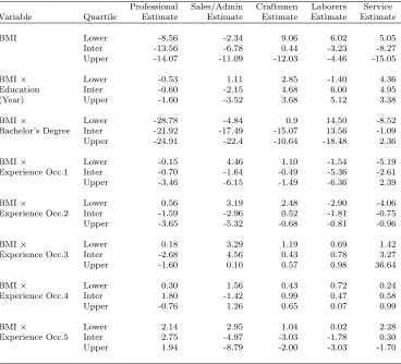
Recall that Bt is the distance between an individual’s BMI and the ‘healthy weight’

boundary of 25. The right column in table 5 shows that higher body weight leads to lower

wages in mentally and socially intensive occupations. The relationship between body mass

and wages in physically intensive occupations is positive. In all three requirements, however,

the point estimates of the interaction effect of BMI and the requirement are greatest in the

upper quartile of the distribution of wages. Because job requirements vary by occupation

and time, the marginal effects of BtJjt do not vary by occupation.

Table 6 contains the occupation specific marginal effects of body weight on wages.

Conditional on requirements, higher body weight is linked to lower wages in Sales and

Admin-istrative Occupations and Professional, Technical and Managerial occupations. The largest

effects are again found in the upper quartile of the wage distribution. In all occupations,

BMI has a negative effect in the upper quartile, although in the Blue collar and service

also linked to lower returns to ’white collar’ experience in nearly all occupations.24 _Fourth,

higher body mass reduces returns to education in white collar occupations. The greatest

effects again occur in the top quartile.

While the marginal effects ofBt and BtJjt on wages are meant to capture the

weight-based wage penalty and wage differential attributed to productivity, respectively, they must

be interpreted with caution. There may be productivity differences that these indices do not

capture. Additionally, the possibility of factors such as persistence in statistical

discrimina-tion prevents me from attributing the lower returns to experience in white-collar occupadiscrimina-tions

to productivity (Lehmann, 2013).

In summary, individuals of high body mass earn lower wages, lower returns to

educa-tion and experience in white collar occupaeduca-tions, and lower wages in socially intensive jobs.

All of these results are largest in the upper quartile of wages. While larger absolute values

of wages will create larger absolute differences in wages between any two groups, the

dif-ference in wages on the basis of body weight is far greater at the mean than the median.

Overall, the results indicate that heavier individuals are much less likely to be observed in

the upper portions of the wage distribution in white collar occupations. This prediction

fits the data. While our best estimates for contemporaneous weight-based wage penalties

are relatively small, the lower returns to experience, education, negative marginal effects of

social requirements and body weight jointly indicate that body weight is an impediment to

career advancement.

6.2

Fixed, Variable, and Switching Costs

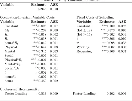
Tables7and8report the estimated cost parameters, including fixed costs of

participat-ing in each occupation and schoolparticipat-ing, switchparticipat-ing costs, and variable costs. The results suggest

that heavier individuals face lower fixed costs of participating in occupations with greater

physical and mental requirements, and higher fixed costs of participating in occupations

24

Table 5: Marginal Effects of Job Requirements on Wages Occupation-Invariant Effects

Requirement Quartile Effect Requirement Quartile Effect *BMI

Physical Lower 46.52 Physical Lower 1.09

Inter 125.86 Inter 9.29

Upper 153.84 Upper 18.85

Mental Lower -2.85 Mental Lower -0.46

Inter 5.01 Inter -2.31

Upper 18.57 Upper -1.75

Social Lower -16.26 Social Lower -1.15

Inter 8.66 Inter -2.05

Upper 48.06 Upper -5.86

Values are in 1983 cents

Table 6: Occupation-Specific Marginal Effects - BMI and Interactions Professional Sales/Admin Craftsmen Laborers Service

Variable Quartile Estimate Estimate Estimate Estimate Estimate

BMI Lower -8.56 -2.34 9.06 6.02 5.05

Inter -13.56 -6.78 0.44 -3.23 -8.27

Upper -14.07 -11.09 -12.03 -4.46 -15.05

BMI× Lower -0.53 1.11 2.85 -1.40 4.36

Education Inter -0.60 -2.15 4.68 6.00 4.95

(Year) Upper -1.60 -3.52 3.68 5.12 3.38

BMI× Lower -28.78 -4.84 0.9 14.50 -8.52

Bachelor’s Degree Inter -21.92 -17.49 -15.07 13.56 -1.09

Upper -24.91 -22.4 -10.64 -18.48 2.36

BMI× Lower -0.15 4.46 1.10 -1.54 -5.19

Experience Occ.1 Inter -0.70 -1.64 -0.49 -5.36 -2.61

Upper -3.46 -6.15 -1.49 -6.36 2.39

BMI× Lower 0.56 3.19 2.48 -2.90 -4.06

Experience Occ.2 Inter -1.59 -2.96 0.52 -1.81 -0.75

Upper -3.65 -5.32 -0.68 -0.81 -0.96

BMI× Lower 0.18 3.29 1.19 0.69 1.42

Experience Occ.3 Inter -2.68 4.56 0.43 0.78 3.27

Upper -1.60 0.10 0.57 0.98 36.64

BMI× Lower 0.30 1.56 0.43 0.72 0.24

Experience Occ.4 Inter 1.80 -1.42 0.99 0.47 0.58

Upper -0.76 1.26 0.65 0.07 0.99

BMI× Lower 2.14 2.95 1.04 0.02 2.28

Experience Occ.5 Inter 2.75 -4.97 -3.03 -1.78 0.30

Upper 1.94 -8.79 -2.00 -3.03 -1.70

that have greater social requirements. Linking with the wage results, heavier individuals

face lower wages and higher fixed costs in socially intensive jobs while the opposite is true

for physically intensive jobs.

Conditional on the requirements of the job, heavier individuals are found to face higher

fixed costs of working in Professional, Technical, and Manager (PTM); Sales, Clerical, and

Administrative (SCA), and Craftsmen occupations. Heavier individuals face lower fixed costs

of working in Laborer occupations. Since nearly all customer facing jobs are found in the Sales

and Administrative category, this result is not inconsistent with a beauty effect (Hamermesh

and Biddle, 1994). The results also suggest that greater body mass leads to higher switching

costs when entering white collar jobs, which are also the most socially intensive. The effects

are twice as strong for PTM occupations ($6,500 at the mean wage) as SCA jobs ($2,700).

Results therefore suggest that body mass affects occupational attainment, which in turn

affects future experience and future wage distributions. This relationship is further explored

in Section 7.

6.3

Weight Transition

The parameter estimates for the body mass transition equation are reported in Table

9. Similar to the results for wages, the marginal effects require additional interpretation.25

Conditional on body mass entering the period, higher wages are associated with lower body

mass in the following period for individuals with a BMI less than 28, but increasing body

mass for those with a BMI greater than 28. The result for the relatively fit people is

consistent with the notion that higher wages garner more resources for investment in health

capital (Grossman, 1972). However, the interaction effect of body mass and wages is positive,

implying that individuals of higher body mass may use those additional resources on less

healthy goods. The estimates for hours exhibit a similar pattern. While an increase in hours

worked leads to lower body mass in the ensuing period, the interaction effect of body mass

25

Table 7: Utility Function Parameters

Variable Estimate ASE

α 0.5948 0.070

Occupation-Invariant Variable Costs Fixed Costs of Schooling

Variable Estimate ASE Variable Estimate ASE

Constant ***-0.823 0.007 Constant ***1.109 0.082

Mt ***-0.237 0.008 (Ed≥ 12) *** 0.373 0.010

Kt ***-0.018 0.002 (Ed≥ 16) **0.902 0.001

Bt ***0.018 0.001 t ***0.306 0.010

hours*Bt ***0.042 0.001 t2 **-0.098 0.038

Physical ***-0.647 0.008 Working ***0.007 0.000 Mental ***-0.345 0.003 Returning ***0.166 0.003 Social ***0.005 0.001

Physical*Bt *** -0.007 0.001

Mental*Bt *** -0.009 0.001

Social*Bt **0.003 0.001

t - 0.002 0.001

hours*t 0.002 0.001 hours ***0.452 0.002

Unobserved Heterogeneity

Table 8: Utility Function Parameters – Switching and Per-period Fixed Costs Occupation Invariant Fixed Costs

Requirement Estimate ASE Requirement* Estimate ASE Requirement* Estimate ASE

t Body Mass

Physical ***1.378 0.030 Physical -0.001 0.000 Physical ***-0.007 0.001

Mental ***0.203 0.028 Mental ***0.014 0.001 Mental *-0.003 0.001

Social ***0.328 0.023 Social ***-0.004 0.001 Social ***0.005 0.001

Occupation Specific Per-Period Fixed Costs

Occupation Professional Sales & Admin Craftsmen Laborers Service

Variable Estimate ASE Estimate ASE Estimate ASE Estimate ASE Estimate ASE Constant ***3.115 0.104 ***0.552 0.034 ***0.712 0.043 ***-0.205 0.008 ***-0.283 0.026 Years of School ***-0.058 0.006 -0.002 0.000 -0.002 0.000 0.000 0.000 ***-0.019 0.002 (Ed≥12) ***-1.115 0.050 ***-0.002 0.000 ***-0.209 0.035 *** -0.499 0.031 ***-0.312 0.032 (Ed≥16) ***-2.707 0.033 ***-1.924 0.048 ***-0.988 0.056 ***0.011 0.002 ***-1.496 0.061 Body Mass ***0.010 0.001 ***0.009 0.002 ***0.035 0.002 ***-0.004 0.000 ***0.004 0.001

t ***0.033 0.003 ***0.024 0.002 *-0.009 0.004 ***0.007 0.000 ***0.039 0.002

Occupation Specific Switching Costs

Occupation Professional Sales & Admin Craftsmen Laborers Service

Variable Estimate ASE Estimate ASE Estimate ASE Estimate ASE Estimate ASE 1[jt−1 = 0] ***1.934 0.051 ***2.351 0.073 ***2.391 0.060 ***1.985 0.055 ***1.649 0.071 1[jt−1 = 1] – – ***0.009 0.001 ***0.035 0.004 ***0.132 0.015 ***0.003 0.000 1[jt−1 = 2] ***0.042 0.003 – – ***0.859 0.082 ***-0.016 0.003 0.000 0.000 1[jt−1 = 3] 0.001 0.000 ***0.899 0.084 – – ***0.042 0.004 ***1.130 0.075 1[jt−1 = 4] ***0.122 0.012 ***0.018 0.004 ***-0.074 0.006 – – ***0.011 0.001 1[jt−1 = 5] 0.000 0.000 ***0.010 0.001 ***0.090 0.009 ***0.010 0.001 – – 1[jt−1 6=j]∗t ***0.100 0.002 ***0.149 0.003 ***0.120 ***0.003 ***0.013 0.003 ***0.198 0.004 1[jt−1 6=j]∗Bt ***0.052 0.004 ***0.024 0.001 ***0.001 0.001 ***-0.007 0.001 ***0.002 0.000

Unobserved Heterogeneity

Factor Loadings -0.256 0.030 0.136 0.045 -0.090 0.027 0.111 0.021 0.008 0.003

Table 9: Parameter Estimates for Body Mass Density

Variable Estimate ASE Variable Estimate ASE

Constant ***12.720 0.229 Physical **0.138 0.051

γ ***-8.840 0.146 Physical*γ ***0.072 0.022

γ2 _{***2.173 0.035 Mental -0.013 0.141}

γ3 _{***0.9953 0.009 Mental*γ -0.008 0.006}

t ***0.023 0.007 Kt 0.016 0.028

t*γ ***0.029 0.003 Kt*γ -0.002 0.012

t2_{/100 **-0.043 0.021 Spouse Inc. (1000’s) -0.002 0.005}

(t2_{/100)*γ ***-0.076 0.009 Spouse Inc.*γ 0.001 0.002}

Body mass ***-0.354 0.006 (hours/10)*Bt ***-0.167 0.031

Body mass*γ ***0.421 0.005 (hours/10)*Bt*γ ***0.059 0.009

(Ed≥12) 0.103 0.091 wage ***1.035 0.045

(Ed≥12)*γ 0.016 0.038 wage*γ 0.018 0.015

(Ed≥16) -0.070 0.055 wage*(hours/10) ***0.009 0.002 (Ed≥16)*γ ***-0.075 0.022 wage*(hours/10)*γ ***0.004 0.001 Married *0.099 0.055 wage*Body mass ***-0.324 0.014 Married*γ **0.56 0.025 wage* Body mass*γ ***-0.036 0.005

hours/10 ***0.621 0.103 FF Index ***-0.017 0.004

(hours/10)*γ *-0.040 0.024 FF Index*γ **-0.005 0.002 hours2_{/100 -0.001 0.006 Crime Index **-0.143 0.056} (hours2/100)*γ -0.002 0.003 Crime Index*γ 0.002 0.006

Unobserved Heterogeneity

Factor Loading 0.202 0.045

and hours is positive. The education dummies corresponding to high school and college

graduation are associated with lower body mass.

Conditional on education, income, unobserved heterogeneity, and age; physically

in-tensive jobs are shown to increase body mass at the low end of the distribution, but have a

negative effect on body mass in the upper portion of the distribution. As the index for

phys-ical requirements is primarily based on strength, it is logphys-ical that slightly-built individuals

might gain some muscle mass. It also follows that very heavy individuals will be most likely

to experience weight loss in response to an increase in physical exertion. The parameters on

mentally intensive work are not statistically significant.

6.4

Model Fit

To assess how well the model fits the observed data, I simulate employment decisions

and wages using the model and the estimated parameters for 10,000 individuals. Initial

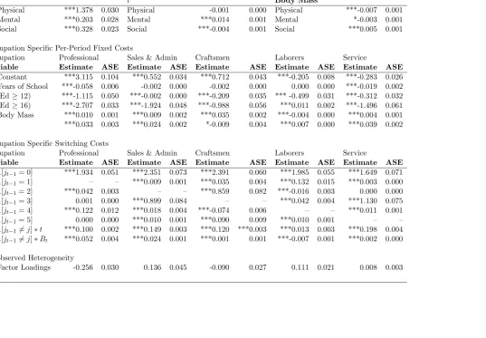
Figure 1: Percentage of Individuals Choosing Each Occupation by Age, Model v. Data

parameters of the model. Details are available in Appendix A. An individual’s “type” is

also drawn randomly using proportions from the estimated distribution of unobserved

het-erogeneity. Figure 1 shows the predicted proportions of chosen occupations by age and the

same proportions from the observed data.

Figure 2 plots the observed and predicted proportions of occupations chosen for the

obese and non-obese by specific age groups. The model predicts the relative differences

be-tween the obese and non-obese well. In each age group in the data, obese workers are less

under the age of 30, obese workers are less likely to be found in sales and administrative

occupations than non-obese workers. The opposite is true in later years. The model predicts

both the levels of and differences between obese and non-obese workers sorting into

crafts-men, laborer, and service occupations. The model mispredicts weight-based differences in

occupational choice in three ways: the model over predicts selection into Craftsmen

occupa-tions, the model over predicts the selection of obese workers into Laborer jobs, and under

predicts the selection of obese workers into service occupations.

Figure3plots the observed and predicted wages for the obese and non-obese by age for

each occupational category. In the white collar occupations where growth in wage disparity

on the basis of weight is common, the model captures the growth in wages for both weight

groups. In the observed data from professional occupations, obese workers make $0.84 per

hour (in 1983 dollars) less than their non-obese counterparts at age 25, and $4.27 less than

non-obese workers at age 45. The model predicts these differences to be $0.67 and $4.42 at

ages 25 and 45 respectively. The model also predicts the growth in the difference in mean

wages as individuals age for Sales, Clerical, and Administrative Occupations. In the data,

obese workers earn $1.42 per hour less than their non-obese counterparts at age 25, and

$3.71 less at age 45. The model predicts these differences to be $1.39 and $4.10 respectively.

As seen in Figure3, the model not only predicts the end points fairly well, but also predicts

the trends in between. The model also predicts wages by weight status for blue collar

occupations, and predicts non-disparities in blue collar occupations, and stable disparity in

service occupations. Note that the scaling is smaller in the bottom three panels of Figure 3

as mean wages in these occupations were lower in both initial values and growth rates over

the sample period. In all occupations, the model over predicts wages for non-obese workers

for the last 2-4 years.

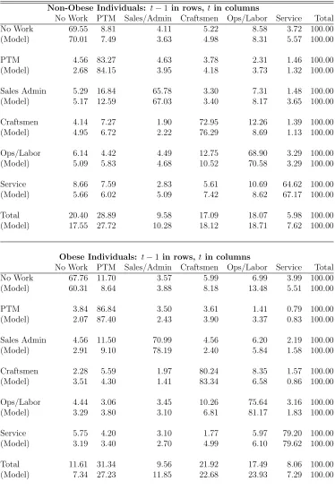
Table 10 contains the observed and predicted transition matrices for obese and

non-obese individuals. The model under predicts persistence in unemployment for non-obese workers,

obese workers from unemployment to laborer work, and under-predicts the transition from

unemployment to professional work. However, as the model over predicts the selection of

obese workers into sales/administrative occupations laborer occupations, this final result is

not surprising.

7

Simulations

Having shown that the estimated model fits the key stylized facts of the observed data,

I conduct a few simulations using the specified model and estimated parameters to illustrate

the dynamic effects of body weight on employment decisions and wages over the life cycle.

I first construct a simulated sample of 10,000 individuals that reflects the distribution of

unobserved heterogeneity and initial conditions for years of schooling body mass. I then

simulate wage offers, employment decisions and weight gain from age seventeen onward.

While the previous section treated the effects of body weight on employment decisions as

separate, they are interrelated. The non-monetary costs of employment affect employment

decisions and subsequent wages. Wage differentials affect employment decision and outcomes.

These simulations serve to show how these different costs and factors work in concert. As

this is a partial equilibrium model, all of these effects should be interpreted in the context

of the individual worker rather than the population.

The first simulation supposes individuals no longer incur any additional switching costs

due to their body weight and evaluates how this increased occupational mobility will affect

employment choices and wages. The results are displayed in Figure4. Since the white collar

occupations were the only ones estimated to have substantial entry frictions due to body

mass, these occupations are the focus of this simulation. Figure 4shows that in the absence

of weight-specific switching costs, the probabilistic gap in choosing Professional, Technical,

and Managerial occupations shrinks by approximately 20 percent. The top left panel shows

Table 10: Occupational Transitional Matrix

Non-Obese Individuals: t−1 in rows,tin columns

No Work PTM Sales/Admin Craftsmen Ops/Labor Service Total No Work 69.55 8.81 4.11 5.22 8.58 3.72 100.00 (Model) 70.01 7.49 3.63 4.98 8.31 5.57 100.00

PTM 4.56 83.27 4.63 3.78 2.31 1.46 100.00 (Model) 2.68 84.15 3.95 4.18 3.73 1.32 100.00

Sales Admin 5.29 16.84 65.78 3.30 7.31 1.48 100.00 (Model) 5.17 12.59 67.03 3.40 8.17 3.65 100.00

Craftsmen 4.14 7.27 1.90 72.95 12.26 1.39 100.00 (Model) 4.95 6.72 2.22 76.29 8.69 1.13 100.00

Ops/Labor 6.14 4.42 4.49 12.75 68.90 3.29 100.00 (Model) 5.09 5.83 4.68 10.52 70.58 3.29 100.00

Service 8.66 7.59 2.83 5.61 10.69 64.62 100.00 (Model) 5.66 6.02 5.09 7.42 8.62 67.17 100.00

Total 20.40 28.89 9.58 17.09 18.07 5.98 100.00 (Model) 17.55 27.72 10.28 18.12 18.71 7.62 100.00

Obese Individuals: t−1 in rows,tin columns

No Work PTM Sales/Admin Craftsmen Ops/Labor Service Total No Work 67.76 11.70 3.57 5.99 6.99 3.99 100.00 (Model) 60.31 8.64 3.88 8.18 13.48 5.51 100.00

PTM 3.84 86.84 3.50 3.61 1.41 0.79 100.00 (Model) 2.07 87.40 2.43 3.90 3.37 0.83 100.00

Sales Admin 4.56 11.50 70.99 4.56 6.20 2.19 100.00 (Model) 2.91 9.10 78.19 2.40 5.84 1.58 100.00

Craftsmen 2.28 5.59 1.97 80.24 8.35 1.57 100.00 (Model) 3.51 4.30 1.41 83.34 6.58 0.86 100.00

Ops/Labor 4.44 3.06 3.45 10.26 75.64 3.16 100.00 (Model) 3.29 3.80 3.10 6.81 81.17 1.83 100.00

Service 5.75 4.20 3.10 1.77 5.97 79.20 100.00 (Model) 3.19 3.40 2.70 4.99 6.10 79.62 100.00

Total 11.61 31.34 9.56 21.92 17.49 8.06 100.00 (Model) 7.34 27.23 11.85 22.68 23.93 7.29 100.00

Figure 4: Counterfactual Results - Elimination of Body Mass Specific Switching Costs

and the hypothetical simulation. The model predicts that an obese worker is 25 percent

less likely than a non-obese worker to choose employment in a professional occupation in his

early thirties. Without weight specific switching costs, an obese male is only 15 percent less

likely to be employed in a professional occupation by age 35. The sharpest reduction in the

attainment gap occurs between ages 30 and 35, when careers are advancing.

The upper panel on the right side shows the effects of the hypothetical policy on

weight-based differences in attaining work in sales, clerical, and administrative occupations.

Without weight-specific switching costs, an obese worker is 10 percent more likely than

a non-obese worker to choose a sales and administrative occupation after age 30. These

occupations are high paying relative to laborer and service occupations, and have lower

social requirements than the professional occupations. The third panel in Figure 4 shows

the growth of the difference in mean real wages between obese and non-obese workers as

predicted by the baseline model and the counterfactual simulation. If an obese individual

experienced no weight-specific barriers to occupational mobility, the expected wage gap

between an obese worker and non-obese worker would decrease by an average of12 percent

The second simulation examines the effects of a one-time exogenous mid-career shock to

an individual’s body weight. Baseline predictions were formed by simulating the model using

the estimated parameters and the observed data. I again predicted occupational choices and

wages using the estimated parameters of the model, but reduced the individual’s Body Mass

Index by one weight class (5 points) at age 35.26 _{The results are displayed below in Figure5.}

The initial change in wages is small (< 4 percent), which is consistent with prior literature

that has found no direct wage penalties’ for body weight. However, by age 45, an individual

who lost a weight class at age 35 is expected to earn 10 percent more than an individual

who did not.

This increase is driven by both a predicted increase in the probability of attaining a

white collar occupation after the shock (see top panels), and increases in expected wages in

those occupations. The model predicts that such an exogenous shock would increase wages

by approximately $1.54 in professional occupations and $.1.37 in sales and administrative

occupations. The individual is