ELEMENTARY WAVE INTERACTIONS IN MAGNETOGASDYNAMICS
1Yujin Liu and Wenhua Sun
School of Science, Shandong University of Technology, Zibo, 255049,
Shandong Province, P. R. China
e-mail: [email protected]
(Received 1 January 2014; after final revision 18 May 2015;
accepted 30 September 2015)
This paper is mainly concerned with the interactions of the elementary waves for the one-dimensional ideal Magnetogasdynamics with transverse magnetic field. By applying the method of the charac-teristic analysis, we obtain constructively the solutions of the all possible wave interactions when the initial data are three piecewise constant states. We find that the result is very different from that of the corresponding case of the conventional gas dynamics. However, the result is consistent with that of the corresponding case for Euler equations when the magnetic field vanishes. Key words : Wave interaction; Riemann problem; magnetogasdynamics; shock wave; rarefaction wave; contact discontinuity.
1. I
NTRODUCTIONIt is well known that Magnetogasdynamics plays a very important role in studying engineering physics
and many other aspects ([1, 4, 8, 9, 10, 13, 14, 19] and the references cited therein) and it is also an
important example of the hyperbolic system’s theory.
One-dimensional inviscid and perfectly conducting compressible fluid, subject to a transverse
magnetic field, is described by the following conservation laws
τ
t−
u
x= 0
,
u
t+ (
p
+
B2
2µ
)
x= 0
,
(
E
+
B2µ2τ)
t+ (
pu
+
B2u
2µ
)
x= 0
,
(1.1)
1
Partially supported by the National Natural Science Foundation of China (No. 11326156, No. 11026048) and partially
under the assumption
B
=
kρ
, where
k
is positive constant [6, 15, 16],
τ
,
u
,
p
,
E
and
B
≥
0
denote the specific volume, velocity, pressure, the specific total energy and transverse magnetic field,
respectively.
E
=
e
+
u22and
e
is specific internal energy. Here
ρ
=
τ1is the density,
µ
is the magnetic
permeability. For the polytropic gas,
e
=
γpτ−1where
γ
is the adiabatic gas constant and
1
< γ <
3
for most gases.
Hu and Sheng [6] studied the system (1.1) with the following initial data
(
τ, p, u
)(
x,
0) = (
τ
±, p
±, u
±)
,
±
x >
0
,
(1.2)
where
τ
±, p
±, u
±are arbitrary constants, and
τ >
0
is the specific volume. They obtained
construc-tively the unique solution of the Riemann problem (1.1) and (1.2) with the characteristic method.
Raja Sekhar and Sharma [15] studied the Riemann problem for one-dimensional unsteady simple
flow of an isentropic, inviscid and perfectly conducting compressible fluid, subject to a transverse
magnetic field
ρ
t+ (
ρu
)
x= 0
,
(
ρu
)
t+ (
ρu
2+
p
+
B2
2
)
x= 0
,
(1.3)
and they obtained the Riemann solutions constructively. Moreover, they discussed the interactions of
the elementary waves.
Shen [16] studied the Riemann problem for (1.3) further and found that the Riemann solutions
converge to the corresponding Riemann solutions of the transport equations by letting both the
pres-sure and the magnetic field vanish.
In [11], we removed the above assumption
B
=
kρ
and mainly consider the Riemann problem of
the one-dimensional unsteady flow of an inviscid, perfectly conducting compressible fluid, subject to
a transverse magnetic field for the magnetogasdynamic system
ρ
t+ (
ρu
)
x= 0
,
(
ρu
)
t+ (
ρu
2+
p
+
B2
2
)
x= 0
,
(
B
)
t+ (
Bu
)
x= 0
,
(1.4)
where the pressure
p
is given by
p
=
Aρ
γfor polytropic gas, A is positive constant and
γ
is the
adiabatic constant.
gas dynamics since the governing equations are highly nonlinear and complicated even for the
one-dimensional flow.
It is noticed that although the governing equations of magnetogasdynamics are more complex
than that of the conventional gas dynamics system, many results are similar except for the contact
discontinuity. Unlike the conventional gas dynamics, where the image of the contact discontinuity in
the space
(
τ, p, u
)
is a straight line parallel to the
τ
-axis and the projection on the plane
(
p, u
)
is a
point, here the contact discontinuity is a plane curve in the space
(
τ, p, u
)
and the projection on the
plane
(
p, u
)
is a straight line parallel to the
p
-axis. It induce that the Riemann solutions are more
complex than that of the conventional gas dynamics.
It is important to study the interactions of the elementary waves not only because of their
signifi-cance in practical applications in magnetogasdynamics system such as comparison with the numerical
and experimental results, but also because of their basic role as building blocks for the theory of
mag-netogasdynamics.
In this paper we are concerned with the wave interactions of the elementary waves of (1.1) with
the following initial data
(
B, ρ, u
)(
x,
0) =
(
B
l, ρ
l, u
l)
,
−∞
< x
≤
x
1,
(
B
m, ρ
m, u
m)
, x
1< x
≤
x
2,
(
B
r, ρ
r, u
r)
,
x
2< x <
∞
,
(1.5)
for arbitrary
x
1, x
2∈
R
.
There are many results for the wave interactions of the elementary waves of the hyperbolic system
and we refer the readers to the references [2, 3, 11, 12, 15, 16, 17].
Based on investigating the important properties of the elementary waves containing the shock
wave, rarefaction wave and the contact discontinuity in the phase plane
(
u, p
)
, we obtain
construc-tively the existence and uniqueness of the solution of the initial value problem (1.1) and (1.5) which
embodies the internal mechanism of this model.
Note that we should deal with the contact discontinuity carefully since it is much more
compli-cated than that of the conventional gas dynamics. We find that the result is very different from that of
the corresponding case of the conventional gas dynamics. However, the result is consistent with that
of the corresponding case for Euler equations when the magnetic field
B
vanishes which indicates
that there is a close connection between the two hyperbolic systems.
The rest of this paper is organized as follows. Section 2 restates the Riemann problem (1.1) and
(1.2) for our later discussions. In Section 3, when the initial date are three pieces of constant states,
the interactions of the elementary waves are considered case by case by investigating the wave curves
in the phase plane
(
u, p
)
and we construct uniquely the solution of the initial value problem (1.1) and
(1.5).
2. P
RELIMINARIESIn this section, we firstly sketch the results of the Riemann problem for (1.1) with the initial data
(1.2), and we refer the readers to [6] for more details.
The system (1.1) can be rewritten, when we consider a smooth solution, as
1
0 0
0
1 0
(
e
+
B2µ2)
τ u e
p
τ
u
p
t
+
0
−
1
0
BBτ
µ
0
1
uBBτ
µ
p
+
B2
2µ
u
τ
u
p
x
= 0
.
(2.1)
It defines the eigenvalues
λ
0= 0
,
λ
±=
±
r
p−epBBτµ +eτ
ep
. If
e
p>
0
and
e
τ+
p >
0
, they are real
and distinct, thus (1.1) is a strictly hyperbolic system. It is easily shown that the characteristic fields
λ
±are genuinely nonlinear and the characteristic field
λ
0is linearly degenerate.
2.1 Rarefaction waves
There are piecewise smooth solutions of (1.1), which are of the form
U
(
xt)
, such that
U
(
x, t
) =
U
l,
xt≤
λ
±(
U
l)
,
U
(
xt)
,
λ
±(
U
l)
≤
xt≤
λ
±(Ur),
U
r,
λ
±(
U
r)
≤
xt.
(2.2)
λ
d
τ
=
−
d(
u
)
,
λ
d
u
= d(
p
+
B2µ2)
,
λ
d(
E
+
B2µ2τ) = d(
pu
+
B2µ2u)
.
(2.3)
Besides the constant state solution
(
τ, p, u
) =
const.
, for the polytropic gas, the forward or
backward rarefaction wave in the
(
τ, p, u
)
space passing though the point
Q
0(
τ
0, p
0, u
0)
is given by
−
→
←
−
R
:
pτ
γ=
p
0τ
0γ,
u
=
u
0±
R
pp0 q
γpτ+B2τ µ
γp
dp.
(2.4)
2.2 Discontinuity
For the system (1.1), the Rankine-Hugoniot (RH) jump conditions are
σ
[
τ
] =
−
[
u
]
,
σ
[
u
] = [
p
+
B2µ2]
,
σ
[
E
+
B2µ2τ] = [
pu
+
B2µ2u]
,
(2.5)
where
[
u
] =
u
r−
u
l, etc.By solving (2.5) we obtain two kinds of discontinuities as follows.
Contact discontinuity:
J
:
σ
= 0
,
[
u
] = [
p
+
B2µ2]
,
(2.6)
and it is easy to see that
J
is a curve with
u
=
Const.
in the
(
τ, p, u
)
space and the projection on the
(
p, u
)
plane is a straight line parallel to the
p
-axis.
For the polytropic gas, the forward or backward shock wave in the
(
τ, p, u
)
space passing though
the point
Q
0(
τ
0, p
0, u
0)
is given by
−
→
←
−
S
:
(p
+
θ
2p
0
+
θ
2(
3B2
2µ
+
B20
2µ
))τ
= (p
0+
θ
2p
+
θ
2(
3B20
2µ
+
B2
2µ
))τ
0,
u
=
u
0±
(p
+
B2
2µ
−
p
0−
B20
2µ
)(
−
τ−τ0
p+B2 2µ−p0−
B20 2µ
)
12,
(2.7)
For convenience and conciseness, denote the projection of
−
→
←
−
R
(
−
→
←
S
−
)
on the
(
τ, p
)
plane and
(
p, u
)
plane by
R
u(
S
u)
and
−
→
←
−
R
τ(
−
→
←
−
S
τ)
, respectively.
Denote the contact discontinuity
J
by
<J
when
p
l< p
r, τ
l< τ
r, and >J
when
p
l> p
r, τ
l> τ
r.For our later discussions, we restate the following properties of the shock wave curves (see
Lemma 3.5. in [6]).
Lemma 2.1 — The wave curve
−
→
S
τ(
Q
0τ)
is concave and monotonically increasing, while
←
S
−
τ(
Q
0τ)
is convex and monotonically decreasing.
In a similar way with Lemma 3.3.7. in [2], we have the following result and the proof is omitted
for simplicity.
Lemma 2.2 — Suppose the point
Q
2∈
−
→
←
−
R
τ(
Q
1)
∪
−
→
←
−
S
τ(
Q
1)
, then the curve
−
→
←
−
S
τ(
Q
1)
does not
intersects with
−
→
←
−
S
τ(
Q
2)
on the side where
p
increases while
−
→
←
−
R
τ(
Q
1)
does not intersects with
−
→
←
−
R
τ(
Q
2)
on the side where
p
decreases.
In order to construct the Riemann problem of (1.1) and (1.2), we denote
←
W
−
−τ(
Q
−τ) =
←
R
−
−τ(
Q
−τ)
∪
←
−
S
−τ(
Q
−τ)
and
−
W
→
+τ(
Q
+τ) =
−
→
R
+τ(
Q
+τ)
∪
−
→
S
+τ(
Q
+τ)
, where
Q
−τand
Q
+τare respectively the
projections of
Q
−and
Q
+on the plane
(
p, u
)
.
Draw
←
W
−
−τ(
Q
−τ)
from
Q
−τand
−
→
W
+τ(
Q
+τ)
from
Q
+τin the plane
(
p, u
)
respectively.
According to the properties of
←
W
−
−τ(
Q
−τ)
and
−
W
→
+τ(
Q
+τ)
, they intersect with each other at most
once. Therefore, there are five cases:
←
W
−
−τ(
Q
−τ)
∩
−
W
→
+τ(
Q
+τ) = (
←
R
−
−τ(
Q
−τ)
∩
−
→
R
+τ(
Q
+τ))
or
(
←
S
−
−τ(
Q
−τ)
∩
−
→
R
+τ(
Q
+τ))
or
(
←
R
−
−τ(
Q
−τ)
∩
−
→
S
+τ(
Q
+τ))
or
(
←
S
−
−τ(
Q
−τ)
∩
−
→
S
+τ(
Q
+τ))
or
∅
.
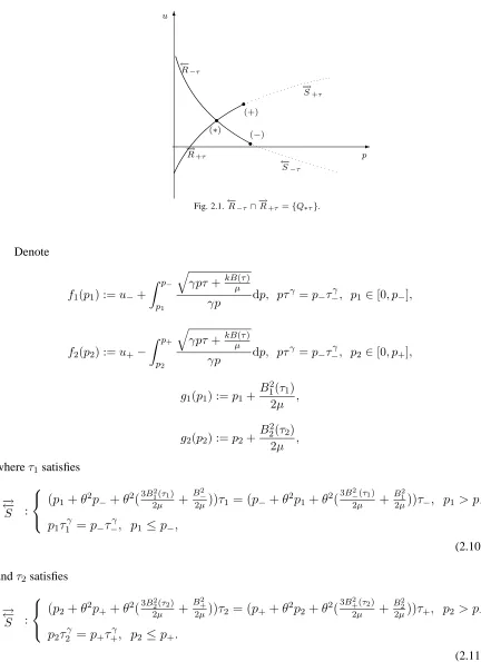
For the last case, we easily know there is a vacuum solution. In what follows, we just need to
consider the first case since the other cases can be studied similarly.
Suppose
←
W
−
−τ(
Q
−τ)
∩
−
→
W
+τ(
Q
+τ) =
←
−
R
−τ(
Q
−τ)
∩
−
→
R
+τ(
Q
+τ) =
{
Q
∗τ}
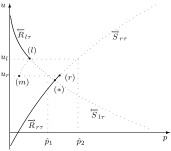
(Fig. 2.1.), we know
there exists
(
p
∗, u
∗)
satisfying
u
∗=
u
−+
Z
p∗p−
q
γpτ
+
kBµγp
d
p, pτ
γ
=
p
−
τ
−γ,
(2.8)
u
∗=
u
+−
Z
p∗p+
q
γpτ
+
kBµγp
d
p, pτ
γ
=
p
-6
r
r r (+)
(−)
p u
(∗)
− →
R+τ
←−
R−τ
− →
S+τ
←−
[image:7.612.78.510.127.722.2]S−τ
Fig. 2.1.←R−−τ∩−→R+τ ={Q∗τ}.
Denote
f
1(
p
1) :=
u
−+
Z
p−p1
q
γpτ
+
kB(τ)µγp
d
p, pτ
γ
=
p
−
τ
−γ, p
1∈
[0
, p
−]
,
f
2(
p
2) :=
u
+−
Z
p+p2
q
γpτ
+
kB(τ)µγp
d
p, pτ
γ
=
p
−
τ
−γ, p
2∈
[0
, p
+]
,
g
1(
p
1) :=
p
1+
B
2 1(
τ
1)
2
µ
,
g
2(
p
2) :=
p
2+
B
2 2(
τ
2)
2
µ
,
where
τ
1satisfies
−
→
←
−
S
:
(p
1+
θ
2p
−+
θ
2(
3B2 1(τ1)
2µ
+
B2 −
2µ
))τ
1= (p
−+
θ
2p
1+
θ
2(
3B2−(τ1)
2µ
+
B2 1
2µ
))τ
−, p
1> p
−,
p
1τ
1γ=
p
−τ
−γ, p
1≤
p
−,
(2.10)
and
τ
2satisfies
−
→
←
−
S
:
(p
2+
θ
2p
++
θ
2(
3B2 2(τ2)
2µ
+
B2 +
2µ
))τ
2= (p
++
θ
2p
2+
θ
2(
3B2+(τ2)
2µ
+
B2 2
2µ
))τ
+, p
2> p
+,
p
2τ
2γ=
p
+τ
+γ, p
2≤
p
+.
Denote
h
1(
p
1) :=
u
−−
s
(
p
1+
B
2 1(
τ
1)
2
µ
−
p
−−
B
2−
2
µ
)(
τ
−−
τ
1)
,
h
2(
p
2) :=
u
++
s
(
p
2+
B
2 2(
τ
2)
2
µ
−
p
+−
B
2+
2
µ
)(
τ
+−
τ
2)
,
where
τ
1satisfies the first equation of (2.10) and
τ
2satisfies the first equation of (2.11).
Let
f
1(
p
1) =
f
2(
p
2)
,
g
1(
p
1) =
g
2(
p
2)
,
(2.12)
f
1(
p
1) =
h
2(
p
2)
,
g
1(
p
1) =
g
2(
p
2)
,
(2.13)
h
1(
p
1) =
f
2(
p
2)
,
g
1(
p
1) =
g
2(
p
2)
.
(2.14)
In [6], the authors proved that only one of the above three equations (2.12), (2.13) and (2.14) is
solvable and the solution is unique, which implies that there exists a unique contact discontinuity
J
joining the two states which are located on
−
→
←
−
R
and
←
−
−
→
S
respectively.
Case 1 :
p
−τ
−γ=
p
+τ
+γ.
In this case, we have
g
1(
p
∗) =
g
2(
p
∗)
, and the Riemann solution is
←
−
R
+
−
→
R
where the symbol
“ + ”
means “followed by”. We notice that for this case there is no contact discontinuity.
Case 2 :
p
−τ
−γ< p
+τ
+γ. In this case, we know that
g
1(
p
∗)
> g
2(
p
∗)
and should look for the
solution in
{
(
p
1, p
2)
|
0
≤
p
1< p
∗, p
2> p
∗}
. There are two possibilities as follows.
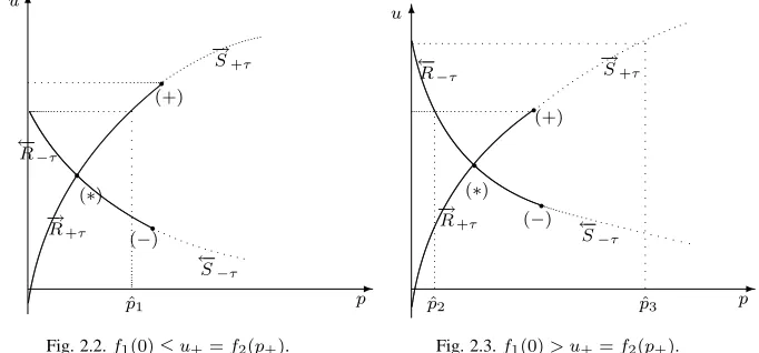
Subcase 2.1 :
f
1(0)
≤
u
+. (Fig. 2.2.)It is obvious that there exists a point
p
ˆ
1∈
(
p
∗, p
+)
such that
f
1(0) =
f
2(ˆ
p
1)
and
g
1(0)
< g
2(ˆ
p
1)
.
It follows that there exists a point
(
p
1, p
2) : 0
< p
1< p
∗, p
∗< p
2<
p
ˆ
1and the Riemann solution
is
←
R
−
+
<J
+
−
→
R
.
Subcase 2.2 :
f
1(0)
> u
+. (Fig. 2.3.)Subcase 2.2.1 : If
g
1(ˆ
p
2)
≤
g
2(
p
+)
, we know that there exists a point
(
p
1, p
2) :
p
ˆ
2≤
p
1<
p
∗, p
∗< p
2< p
+and it follows that the Riemann solution is
←
R
−
+
<J
+
−
→
R
.
Subcase 2.2.2 : If
g
1(ˆ
p
2)
> g
2(
p
+)
, similarly we obtain that there exists a point
(
p
1, p
2) : 0
<
p
1<
p
ˆ
2, p
+< p
2<
p
ˆ
3and the Riemann solution is
←
R
−
+
J
<+
−
→
S
, where
p
ˆ
3∈
(
p
+,
+
∞
)
satisfying
f
1(0) =
h
2(ˆ
p
3)
.
-
-6 6
(+)
(∗)
− →
R+τ (−)
←−
S−τ
←−
R−τ
− →
S+τ
p u
(+)
(−)
ˆ p2
ˆ
p1 pˆ3
− →
S+τ
←−
S−τ
− →
R+τ
←−
R−τ
(∗)
[image:9.612.152.493.246.405.2]p u
Fig. 2.2.f1(0)≤u+=f2(p+). Fig. 2.3.f1(0)> u+=f2(p+). q
q
q q
q
q
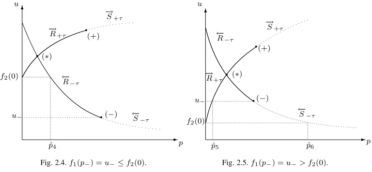
Case 3 :
p
−τ
−γ> p
+τ
+γ. In this case, we know that
g
1(
p
∗)
< g
2(
p
∗)
and should look for the
solution in
{
(
p
1, p
2)
|
p
1> p
∗,
0
≤
p
2< p
∗}
. We divide it into two subcases as follows.
Subcase 3.1 :
u
−≤
f
2(0)
(Fig. 2.4.)
It is obvious that there exists a point
p
ˆ
4∈
(
p
∗, p
−)
such that
f
1(ˆ
p
4) =
f
2(0)
and
g
1(ˆ
p
4)
> g
2(0)
.
And we get the Riemann solution
←
R
−
+
>J
+
−
→
R
.
Subcase 3.2 :
u
−> f
2(0)
(Fig. 2.5.)
Since there exists a point
p
ˆ
5∈
(0
, p
∗)
such that
f
2(ˆ
p
5) =
u
−, we divide it into two subcases.
Subcase 3.2.1 : If
g
1(
p
−)
≥
g
2(ˆ
p
5)
, similarly as the above discussions there exists a point
(
p
1, p
2) :
p
∗< p
1< p
−,
p
ˆ
5≤
p
2< p
∗and the Riemann solution is
←
R
−
+
>
J
+
−
→
R
.
Subcase 3.2.2 : If
g
1(
p
−)
< g
2(ˆ
p
5)
, since there exists a point
(
p
1, p
2) :
p
−< p
1<
p
ˆ
6,
0
<
p
2<
p
ˆ
5, the Riemann solution is←
S
−
+
>J
+
−
→
R
, where
p
ˆ
6satisfies
h
1(ˆ
p
6) =
f
2(0)
.
6
-6
-u
p u
p f2(0)
u− (−)
(+)
ˆ p4
− →
R+τ
− →
S+τ
←−
R−τ
←−
S−τ
(∗)
←−
R−τ
←−
S−τ
− →
R+τ
− →
S+τ
(∗) (+)
(−) u−
ˆ
p5 pˆ6
[image:10.612.175.559.140.318.2]f2(0)
Fig. 2.4.f1(p−) =u−≤f2(0). Fig. 2.5.f1(p−) =u−> f2(0). q
q
q
q q
q
Theorem 2.1 — For any initial constant states
U
−and
U
+, there exists uniquely the entropy
solution of the Riemann problem (1.1) and (1.2).
3. I
NTERACTIONS OF THEE
LEMENTARYW
AVESNow we consider the kinds of interactions of the elementary waves obtained from the Riemann
prob-lem (1.1) and (1.2). We divide the discussions into two cases: the interactions of the eprob-lementary
waves containing no
R
and the interactions of the elementary waves containing
R
.
3.1 Interactions of the elementary waves containing no
R
In this case, we discuss the wave interactions case by case and can obtain the global solution by
solving a new Riemann problem.
Case (i) :
−
→
S
J
>.
Since
−
→
S
rτ(
Q
r) :
u
=
u
r+
q
(
p
+
B22µ
−
p
r−
B2r
2µ
)(
τ
r−
τ
)
,
−
→
S
mτ(
Q
m) :
u
=
u
m+
q
(
p
+
B2µ2−
p
m−
B2 m
2µ
)(
τ
m−
τ
)
,
where
B
r=
τkr,
B
m=
τkmand
u
m=
u
r,
p
m+
B2 m
2µ
=
p
r+
B2r
2µ
. From the properties of the contact
discontinuity, we have
τ
m> τ
r⇔
B
m< B
r, it follows that the curve−
→
S
rτ(
Q
r)
lies always above
the curve
−
→
S
mτ(
Q
m)
. Thus,
−
→
S
rτ(
Q
r)
intersects with
←
−
R
lτ(
Q
l)
at
Q
∗τwhere a new Riemann problem
is formed. In order to construct the solution of this new Riemann problem, we discuss as follows.
Case 1 :
τ
∗l< τ
∗r. In this case,
g
1(
p
∗)
> g
2(
p
∗)
and we should seek a solution in
{
(¯
p
1,
p
¯
2)
|
0
<
¯
[image:10.612.117.554.531.674.2]It is obvious that there exists a point
p
ˆ
1∈
(
p
∗,
+
∞
)
which satisfies
f
1(0) =
h
2(ˆ
p
1)
and
0 =
g
1(0)
< g
2(ˆ
p
1)
. It follows that there exists a point
(¯
p
1,
p
¯
2) : 0
<
p
¯
1< p
∗, p
∗<
p
¯
2<
p
ˆ
1and the
solution is given by
−
→
S
>J
→
←
R
−
<J
−
→
S
.
Case 2 :
τ
∗l=
τ
∗r. Since there is no contact discontinuity of the new Riemann solution in this
case, the state
Q
lis connected to the state
Q
rby the state
Q
∗directly and we obtain that the solution
is
−
→
S
J
>→
←
R
−
−
→
S
.
Case 3 :
τ
∗l> τ
∗r. This means that
g
1(
p
∗)
< g
2(
p
∗)
, i.e.,
p
∗l+
B2 ∗l
2µ
< p
∗r+
B2∗r
2µ
, where
B
∗l=
τk∗l,
B
∗r=
τk∗r.
In view of
u
l> u
r, if there is a contact discontinuity
(¯
p
1,
p
¯
2)
of the solution for the new Riemann
problem, we know that the following equality
¯
p
1+
¯
B
2 12
µ
= ¯
p
2+
¯
B
2 22
µ
,
(3.1)
holds, where
p
¯
1> p
∗,
0
<
p
¯
2< p
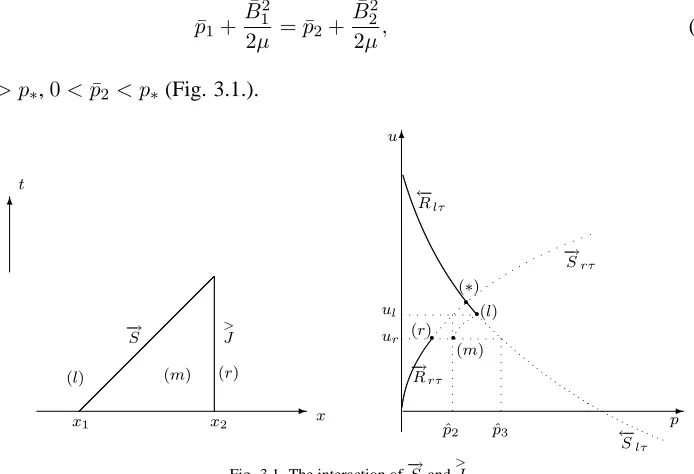
∗(Fig. 3.1.).
6
-p u
− →
Srτ
←−
Rlτ
←−
Slτ
− →
Rrτ
(l) (r)
(∗)
ˆ p3
[image:11.612.148.495.332.569.2]ˆ p2
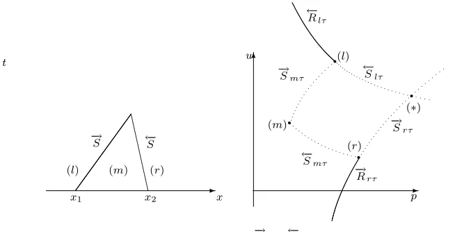
Fig. 3.1. The interaction of−→S and >
J.
ul
ur
(m)
-6
(l) (m) (r)
x1 x2 x
t
− →
S >J
q q q
q
Subcase 3.1 :
g
1(
p
l)
≥
g
2(ˆ
p
2)
, where
p
ˆ
2is determined by
u
l=
u−
→Srτ(ˆ
p
2)
, i.e., we choose
p
ˆ
2such
that the value of
u
along the curve
−
→
S
rτas
p
= ˆ
p
2equals to the value of
u
l. Therefore there exists a
point
(¯
p
1,
p
¯
2) :
p
∗<
p
¯
1< p
l,
p
ˆ
2<
p
¯
2< p
∗and the solution lies between
u
land
u
∗which is given
by
−
→
S
>J
→
←
R
−
>J
−
→
S
.
Subcase 3.2 :
g
1(
p
l)
< g
2(ˆ
p
2)
. On the other hand, we have
ˆ
p
3+
B
ˆ
232
µ
> p
r+
B
2r
where
p
ˆ
3is determined by
u
←−Slτ(ˆ
p
3) =
u
r. In fact, due to
p
m+
B2 m
2µ
=
p
r+
B2r
2µ
,
u
m=
u
r=
u
(ˆ
p
3) =
u
l−
s
(ˆ
p
3+
ˆ
B
2 32
µ
−
p
l−
B
2l
2
µ
)(
τ
l−
τ
ˆ
3)
,
and
u
m=
u
l−
s
(
p
l+
B
2 l2
µ
−
p
m−
B
2m
2
µ
)(
τ
m−
τ
l)
,
where
p
ˆ
3> p
l> p
m. From Lemma 2.1., dτdp<
0
holds for
←
−
S
which yields that
τ
ˆ
3< τ
l< τ
m. Itfollows that
ˆ
p
3+
ˆ
B
2 32
µ
> p
l+
B
2l
2
µ
> p
m+
B
2m
2
µ
=
p
r+
B
2r
2
µ
,
that is to say, (3.2) holds.
Hence there exists a point
(¯
p
1,
p
¯
2) :
p
l<
p
¯
1<
p
ˆ
3, p
r<
p
¯
2<
p
ˆ
2and the solution is described
by
−
→
S
>
J
→
←
S
−
>J
−
→
S
.
Similarly, the interaction between
<J
and
←
S
−
can also be obtained and here omitted.
Theorem 3.1 — When a shock collides with a contact discontinuity which is of a jump increase in
density in the propagating direction of the shock, the shock will cross the contact discontinuity at once
and a new rarefaction wave or a new shock wave propagating in the opposite direction will appear.
Furthermore, after the interaction the contact discontinuity may appear or disappear.
Case (ii) :
−
→
S
J
<. Similar discussions as the above case, it follows that the curve
−
→
S
mτ(
Q
m)
lies
always above the curve
−
→
S
rτ(
Q
r)
. Thus, there are two possibilities:
←
S
−
lτ(
Q
l)
intersects with
−
→
S
rτ(
Q
r)
at
Q
∗τwhere a new Riemann problem is formed, or
←
−
S
lτ(
Q
l)
intersects with
−
→
R
rτ(
Q
r)
at
Q
∗τwhere
a new Riemann problem is formed. In what follows, we construct the solution of the new Riemann
problem as follows.
Case 1 :
p
ˆ
1≥
p
r, where
p
ˆ
1satisfies
u
r=
u←
S−lτ(ˆ
p
1)
. In this case, we know that
Q
∗τ∈
←
−
S
lτ(
Q
l)
∪
−
→
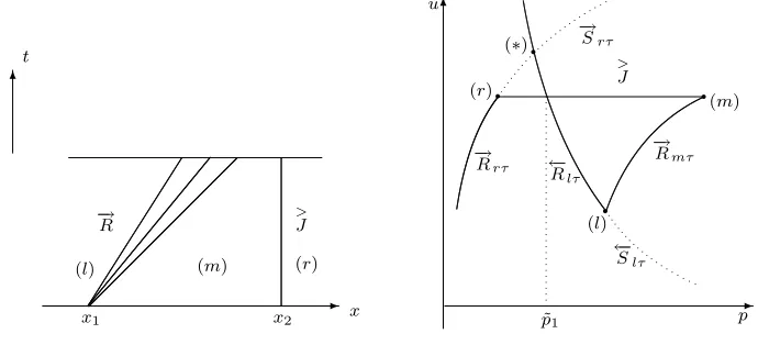
-6
(l) (m) (r)
x1 x2
−→
S <J
x t
-6
u
p
− →
Srτ
←−
Slτ
− →
Rrτ
←−
Rlτ
(l) (∗)
(r)
ˆ p3
[image:13.612.135.496.138.284.2]ˆ p2
Fig. 3.2. The interaction of−→Sand <
J,pˆ1≥pr.
ˆ p1
ur
ul
(m)
q q q q
Subcase 1.1 :
τ
∗l< τ
∗r. This means thatg
1(
p
∗)
> g
2(
p
∗)
. If there exists a contact discontinuity
(¯
p
1,
p
¯
2)
of the new Riemann problem, (3.1) must hold. There are two possibilities.
Subcase 1.1.1 :
g
1(
p
l)
≤
g
2(ˆ
p
2)
, where
p
ˆ
2is determined by
u
l=
u
−→Srτ(ˆ
p
2)
.
(3.3)
Therefore the solution lies between
u
land
u
∗and the result is
−
→
S
J
<→
←
S
−
<J
−
→
S
.
Subcase 1.1.2 :
g
1(
p
l)
> g
2(ˆ
p
3)
. On the other hand,
0 =
g
1(0)
< g
2(ˆ
p
3)
holds obviously, where
ˆ
p
3is determined by
u←
R−lτ(Ql)
(0) =
u−
→Srτ(ˆ
p
3)
. It follows that there exists
(¯
p
1,
p
¯
2)
which satisfies
0
<
p
¯
1< p
l,
p
ˆ
2<
p
¯
2<
p
ˆ
3and
−
→
S
<J
→
←
R
−
J
<−
→
S
.
Subcase 1.2 :
τ
∗l=
τ
∗r. There is no contact discontinuity of the new Riemann solution and theresult is given by
−
→
S
<J
→
←
S
−
−
→
S
.
Subcase 1.3 :
τ
∗l> τ
∗r.This means that
g
1(
p
∗)
< g
2(
p
∗)
. On the other hand, it is evident that
p
r+
B
2 r2
µ
=
p
m+
B
m22
µ
<
p
ˆ
1+
ˆ
B
122
µ
.
It yields that there exists
(¯
p
1,
p
¯
2) :
p
∗<
p
¯
1<
p
ˆ
1, p
r<
p
¯
2< p
∗such that (3.1) holds. Thus, we
have
−
→
S
<J
→
←
S
−
>J
−
→
S
.
6
-p u
− →
Srτ
− →
Rrτ
←−
Slτ
←−
Rlτ
ˆ p2
ˆ p1
(l)
[image:14.612.287.458.141.292.2](r) (∗)
Fig. 3.3. The interaction of−→S and <
J,pˆ1< pr.
ul
ur
(m) qq
q q
Subcase 2.1 :
τ
∗l< τ
∗r. This means thatp
∗l+
B2 ∗l
2
> p
∗r+
B2∗r
2
. Therefore, we have obviously
that
ˆ
p
1+
ˆ
B
2 12
µ
> p
m+
B
2m
2
µ
=
p
r+
B
2r
2
µ
.
and there is no solution between
u
∗and
u
r.Subcase 2.1.1 :
g
1(
p
l)
≤
g
2(ˆ
p
2)
, where
p
ˆ
2satisfies (3.3). Thus, there exists a point
(¯
p
1,
p
¯
2)
which
satisfies
p
l<
p
¯
1< p
∗, p
r<
p
¯
2<
p
ˆ
3and
−
→
S
<J
→
←
S
−
<J
−
→
S
.
Subcase 2.1.2 :
g
1(
p
l)
> g
2(ˆ
p
2)
. The solution lies between 0 and
u
land
−
→
S
<J
→
←
R
−
<J
−
→
S
.
Subcase 2.2 :
τ
∗l=
τ
∗r. There is no contact discontinuity of the new Riemann solution and theresult is
−
→
S
J
<→
←
S
−
−
→
R
.
Subcase 2.3 :
τ
∗l> τ
∗r. This means that
p
∗l+
B2 ∗l
2µ
< p
∗r+
B2∗r
2µ
. It is obvious that
0
<
p
ˆ
4+
ˆ B24
2µ
,
where
p
ˆ
4satisfies
u−
→Rrτ(Qr)(0) =
u←
−Slτ(Ql)
(ˆ
p
4)
. Therefore there exists
(¯
p
1,
p
¯
2) : ˆ
p
1<
p
¯
1<
p
ˆ
4,
0
<
¯
p
2< p
rsuch that (3.1) holds which indicates that
−
→
S
<J
→
←
S
−
J
>−
→
R
.
Similarly, the interaction between
>J
and
←
S
−
can be investigated and omitted for simplicity.
Theorem 3.2 — When a shock collides with a contact discontinuity which is of a jump decrease
in density in the propagating direction of the shock, the shock will cross the contact discontinuity at
once or a new rarefaction wave will appear, and after the interaction the contact discontinuity may
appear or disappear. Furthermore, a new shock wave or a new rarefaction wave propagating in the
Case (iii) :
−
→
S
←
S
−
. In this case, it is obvious that
−
→
S
will intersect with
←
−
S
in a finite time and
a new Riemann problem is formed. From Lemma 2.2., we know that
←
S
−
τ(
Q
l)
does not intersect
with
←
−
S
τ(
Q
m)
and
−
→
S
τ(
Q
r)
does not intersect with
−
→
S
τ(
Q
m)
, respectively. It follows that
Q
∗∈
←
−
S
τ(
Q
l)
∪
−
→
S
τ(
Q
r)
(Fig. 3.4.) and we construct the solution as follows.
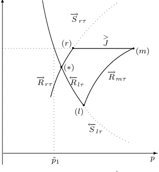
-6
(l) (m) (r)
x1 x2
− →
S ←S−
x t
-6
u
[image:15.612.138.465.206.373.2]p
Fig. 3.4. The interaction of−→S and←S−.
(m)
(l)
(r)
(∗)
− →
Smτ
←−
Smτ
←−
Rlτ
←−
Slτ
− →
Rrτ
− →
Srτ
q
q
q
q
Case 1 :
τ
∗l> τ
∗r. In this case,g
1(
p
∗)
< g
2(
p
∗)
and we should seek a solution in
{
(
p
1, p
2)
|
p
1>
p
∗,
0
< p
2< p
∗}
. Obviously, there exist
p
ˆ
1and
p
ˆ
2which satisfies respectively that
u
r=
u
←S−lτ(ˆ
p
1)
,
p
ˆ
1∈
(
p
∗,
p
ˆ
2)
and
u−
→Rrτ(0) =
u←
−Slτ
(ˆ
p
2)
,
p
ˆ
2>
p
ˆ
1> p
∗.
Subcase 1.1 :
g
1(ˆ
p
1)
≥
g
2(
p
r)
. From the continuity of the wave curves, we know there exists a
point
(¯
p
1,
p
¯
2)
such that
p
∗<
p
¯
1<
p
ˆ
1, p
r<
p
¯
2< p
∗, and the solution is
−
→
S
←
S
−
→
←
S
−
>
J
−
→
S
.
Subcase 1.2 :
g
1(ˆ
p
1)
< g
2(
p
r)
. Similarly, we know there exists a point
(¯
p
1,
p
¯
2)
satisfying
p
ˆ
1<
¯
p
1<
p
ˆ
2and
0
<
p
¯
2< p
rand the result is described by
−
→
S
←
S
−
→
←
S
−
>J
−
→
R
.
Case 2 :
τ
∗l=
τ
∗r. In this case,g
1(
p
∗) =
g
2(
p
∗)
and there is no contact discontinuity of the new
Riemann solution, the state
Q
lis connected to the state
Q
rby the state
Q
∗directly and we obtain that
the solution is
−
→
S
>J
→
←
S
−
−
→
S
.
Case 3 :
τ
∗l< τ
∗r. This means that
g
1(
p
∗)
> g
2(
p
∗)
and we should seek solution in
{
(¯
p
1,
p
¯
2)
|
0
<
¯
p
1< p
∗,
p
¯
2> p
∗}
. It is easily shown that there exist
p
ˆ
3and
p
ˆ
4which satisfies respectively that
u
l=
u−
→Srτ