.A thesis
submitted for the Degree of
Doctor of Philosophy in Computer Science in the
University of Canterbury
by
S.A. Freeth
TO
ACKNOWLEDGEMENTS
I wish to thank Professor J.P. Penny for accepting me as a research student, my supervisors Dr. Tadeo Takaoka for introducing me to the subject, and Dr. B.J. McKenzie for his guidance and encouragement in preparing this thesis. I would also like to thank Mr. A.M. Moffat for many helpful comments on the drafts.
I wish to th~nk Mr. G. Smith of Gabites, Porter and Partners (CH-CH) Ltd., for the opportunity of working with transportation networks 'in the real world' and also Mr. G. Bellis who ran the transportation models. I wish to thank the Christchurch Transport Board for permission to use the map in Appendix A.
I wish to thank Mr.
c.
Hadlee for drafting many of the graphs.ABSTRACT
Two compression methods for representing graphs are presented, in conjunction with algorithms applying these methods.
A decomposition technique for networks that can be generated in O(m) time is presented. The components of the decomposition and the shortest path matrix of the compressed network can be used to find the shortest path between any pair of vertices in the original network in linear time.
A compression method for boolean matrices and a method for applying the compression to boolean matrix multiplication is. developed. The algorithms have an expected running time of O(n2*log2n). From this compression method a simple heuristic that may be applied to any algorithm for boolean matrix multiplication has been developed. This heuristic will improve the average running time of boolean matrix multiplication algorithms.
An order of magnitude analysis of the results published by Loukakis and Tsouris [1981], on the efficiency of algorithms for finding all maximal independent sets of a graph has been .Performed. This analysis showed that their conclusions, which are based on a direct comparison of the running times of the algorithms, do not take into account implementation factors.
-CHAPTER 1:
CHAPTER 2: 2.1 2.2 2.3 2.4 2.5 2.6 2.7
CHAPTER 3 : 3.1 3.2 3.3 3.4 3.5
CHAPTER 4:
4.1 4.2 4.3 4.4 4.5 4.6 4.7 4.8
TABLE OF CONTENTS
INTRODUCTION
BACKGROUND Introduction Graphs
Representation of Graphs Graphs and Boolean Matrices Trees
Probability Distribution Maximal Independent Sets
A SURVEY OF GRAPH REPRESENTATION Introduction
Representation of Graphs Graph Decomposition
Graph Homomorphism Summary
A DECOMPOSITION ALGORITHM FOR SHORTEST PATHS ON NETWORKS Introduction
Decomposition of a Network A Compressed Network
Selected Shortest Paths Analysis of Complexity
CHAPTER 5: 5.1 5.2 5.3 5.4 5.5 5.6 5.7 5.8 5.9
CHAPTER 6:
6.1 6.2 6.3 6.4 6.5 6.6
CHAPTER 7:
REFERENCES APPENDICES A: B: C: Page
BOOLEAN MATRIX MULTIPLICATION 77
Introduction 77
Tree Summation Methods 78
The Algorithm 87
Alternative Summation Sizes 95
Analysis of Complexity 96
Results 104
Comparison with Other Algorithms 111 Applying a Summation Heuristic to
Other Algorithms 122
Summary 127
AN EFFICIENT AVERAGE TIME ALGORITHM FOR THE GENERATION OF ALL MAXIMAL INDEPENDENT SETS OF A GRAPH
Introduction
The Algorithm of Tsukiyama, Ide, Ariyoshi and Shirakawa
Modifications to the Algorithm Results
Comparisons with Other Algorithms Summary
CONCLUSION
Shortest Paths
Boolean Matrix Multiplication Maximal Independent Sets
Definition 2.1 2.2 2.3 2.4 2.5 2.6 2.7 2.8 2.9 2.10 2.11 2.12 2.13 2.14 2.15 2.16 2.17 2.18 2.19 2.20 2.21 2.22 2.23 2.24 2.25
LIST OF DEFINITIONS
Graph
Adjacent Vertices Degree of a Vertex Subgraph
Path on a Graph Simple Path Connected Graph Polygon
Digraph Self Loop
Parallel Edges Network
Path on a Network Isomorphic Graphs Automorphism
Homomorphism
Components of a Graph Node of a Graph
Branches of a Graph Homeomorphism
Vertex Adjacency Matrix Incidence Matrix
Adjacency List Edge List
Closed Semiring
Definition 2.26 2.27 2.28 2.29 2.30 2.31 2.32 4.1 4.2 4.3 4.4 4.5 4.6 4.7 5.1 5.2 Tree
Parent, Child, Ancestor, Descendent Depth, Height, Level
Ordered Tree, Binary Tree, Log Tree Traversal, Depth First, Breadth First Graph Probability Distributions
Maximal Independent Set, Clique Simple Vertices, Link Vertices Branches of a Network
Forward and Backward Paths Decomposition of a Network Composition
Link Edge
Compressed Network Partition Series
Partition Value and Partition Size
LIST OF THEOREMS
Theorem Page
4.1 A Branch Intersects with
<=
2 Link Vertices 424.2 Isomorphism of a Graph and its Branch Graph 43
4.3 Existance of a Decomposition 43
4.4 Unique and Irreducible Decomposition 44
4.5 Reconstruction of the Original Networ5 From the Decomposition
4.6
5.1
Number of Edges in the Compressed Network
Relationship between Boolean Matrix
Multiplication and Summation of Integers
5.2 Partial Sum Relationship between Boolean Matrix Multiplication and Summation of
Integers
43
48
79
LIST OF ALGORITHMS
Algorithm Page
4.1 Generating the Compressed Network and the Shortest Paths of the Components of the Decomposition
4.2 Generating the Compressed Network and the Shortest Paths of the Components of the
49
Decomposition, with Full Data Structures 54
4.3
4.4
Outline of Algorithm for Generating a Shortest Path
Generating the Shortest Paths
5.1 Outline of Algorithm for Boolean Matrix Multiplication
5.2
5.3
Outline of Procedure Tree scan using Depth First Search
Outline of Procedure Tree scan using Breadth First Search
5.4 Terminating Conditions added to the Outline of Procedure Tree scan using Depth First Search
5.5 Terminating Conditions Added to the
Outline of Iterative Procedure Tree scan using Breadth First Search
5.6 Full Algorithm for Boolean Matrix Multiplication using Binary Summation
57
64
87
88
89
90
91
Algorithm Page
6.1 Algorithm of Tsukiyama, Ide, Ariyoshi and Shirakawa
6.2 Modified Algorithm of Tsukiyama, Ide, Ariyoshi and Shirakawa
B.l Takaoka Data Compression Algorithm
B.2 Initialisation of Lists for Takaoka Indexing Algorithms
B.3 Takaoka HAVB Algorithm
B.4 Takaoak VAHB Algorithm
B.S Takaoka HAHB Algorithm
132
144
195
197
198
198
LIST OF FIGURES
Figure
2.1 A Graph on 10 Vertices and 19 Edges
2.2 A Digraph on 10 Vertices and 17 Edges
2.3 Adjacency Matrix and Incidence Matrix
2.4 Adjacency List and Edge List
2.5 Maximal Independent Sets
3.1 The Complexity Hierarchy
4.1 A Portion of A Transportation Network
4.2 Two Branches in the Network
4.3 A Portion of the Compressed Network
4.4 Shortest Paths in the Components of the
Decomposition
4.5 Data Structure of Partial Costs for
Components of the Decomposition
4.6 Shortest Paths for Vertices in the
Same Component
4.7 Shortest Paths in a Polygon
4.8 Shortest Path Between Two Vertices
4.9 Graph of t +u Versus t as t Increases 2 From 0 to n
Page
7
10
14
15
23
30
40
41
47
52
53
59
61
62
Figure
5.1 Two Example Matrices
5.2 Binary Summation Partition Series on Two Matrices
5.3 Summation Values of a Binary Summation Partition Series
5.4 Summation Sizes of a Binary Summation Partition Series
5.5 Alternative Recursion Structures
5.6 Summation Values
5.7 Rows and Columns Causing Worst Case Performance
5.8 Number of Procedure Calls Versus Density
Page
80
84
85
85
86
94
99
of ' l ' s in Matrix for Breadth First Search 107
5.9 Number of Procedure Calls Versus Density
of ' l ' s in Matrix for Depth First Search 108
5.10
5.11
5.12
5.13
Maximum Number of Procedure Calls Versus Number of Vertices for All Algorithms
Maximum Number of Procedure Calls Per
2
n *depth Versus n
Running Time Improvements Using Out of Loop Heuristic
Running Time For Elementary and Compression Algorithms
110
112
117
Figure
5.14 Running Time For Indexing Algorithms
5.15 Scale Representation of the
5.16
5.17
6.1
6.2
6.3
Running Times For Algorithms Using the
Summation Heuristic
Running Time For Algorithms With
Summation Heuristic
. . 2
Runn1ng T1me per n Versus Log 2n
For All Algorithms
Generation of Maximal Independent Sets
Using the Original Algorithm
Possible Recursion Trees
Generation of Maximal Independent Sets
Using the Modified Algorithm
6.4 Running Time For Original and Modified Algorithms Versus Number of Maximal
Independent Sets
6.5 Time per Maximal Independent Set Versus Ratio of Procedure Calls For The Original
Page
121
123
124
126
133
140
143
149
Algorithm 152
6.6 Time per Maximal Independent Set Versus Ratio of Prodecure Calls For The Modified
Algorithm 153
6.7 Change In Running Time Versus Change In The
Figure
6.8
6.9
6.10
6.11
6.12
A.l
Time per Maximal Independent Set Versus Number of Vertices For Original and Modified Algorithms
Time per Maximal Independent Set Versus Number of Edges
Time per Maximal Independent Set Versus Number of Vertices For Tsukiyama et al
Page
156
158
Algorithm Reported by Loukakis and Tsouris 163
Time per Maximal Independent Set Versus Number of Vertices For Bron-Kerbosch and Loukakis-Tsouris Algorithms Reported by Loukakis and Tsouris
Time per Maximal Independent Set Versus Number of Vertices For Bron-Kerbosch and
165
Loukakis-Tsouris Algorithms 166
LIST OF TABLES
Table Page
B.l Comparison of Tree Sizes 186
B.2 Parameters of Average Case Test Data 187
B.3 Results of the Use of Different Tree Formats for Log
2n Summation Algorithms 188
B.4
B.5
Comparison of Results for Tree Summation Algorithms
Parameters of Test Data for Comparison of Boolean Matrix Multiploication Algorithms
B.6 Effectiveness of the 'Out of Loop' Heuristic
B.7
B.8
Results for Elementary and Compression Algorithms
Results for Indexing Algorithms
B.9 Results for Algorithms with Summation Heuristic
C.l Worst Case Test Data
C.2 Test Results for Worst Case
C.3 Time per Maximal Independent Set for Worst Case Test Data
C.4 Average Case Te$t Data
189
190
191
192
193
194
201
201
202
Table
c.s
C.6
C.7
c.s
Distribution of Maximal Independent Sets In Average Case Test Data
Test Results For Average Case Data
Improvement in Running Time Achieved by Modified Algorithm
Time per Maximal Independent Set
C.9 Summary of the Number of Rercursive Calls for Average Case Test Data
C.l0
C.ll
C.l2
C.l3
Test Results for Worst Case
Time per Maximal Independent Set For Worst Case Data
Test Results for Average Case Data For All Algorithms
Time per Maximal Independent Set or Clique
Page
204
206
206
207
208
209
210
210
CHAPTER 1
INTRODUCTION
"Although algorithmic graph theory was started by Euler, if not earlier, its development in the last ten years has been dramatic." [Even, 1979]
Graph theory has become recognised as a suitable paradigm for embedding many problems from engineering and science, and therefore algorithms for the solution of graph problems have been i n t e n s i v e l y s t u d i e d . E f f i c i e n t data representations are as important as the techniques used in algorithm design.
Examination of graph algorithms shows, in almost all cases, that the complexity is dependent on the choice of graph representation. Various constraints, for example the type of operation to be performed, determine the most appropriate graph representation for any particular graph problem. It is
~.~
possible1 no single representation will provide a globalsolution for the representation of graphs for all graph algorithms. However, the reported successes, from applying new data structures, in the development of new and efficient algorithms suggests graph representations are worthy of further investigation. Carre [1979] states:
"Since 1970, computer scientists have made important contributions to graph theory • • • they have achieved remarkable improvements in the performance of graph algorithms, mainly through
the clever manipulation of data structures."
While no formal theory exists as a basis for selecting and applying graph representations, continuing research in this area has led to improved algorithms for individual graph problems.
The following organisation has been used in this thesis.
Chapter 2 presents the background of graph theory and terminology used in this thesis. Traditional graph representations and the theoretical relationship between directed graphs and boolean matrices is described. Trees play an extremely important role in algorithm design)so, although they are a class of graph, it is their application to algorithm design that has been considered in this thesis. A probability distribution for graphs is described so that the expected behaviour of algorithms which accept graphs as input may be analysed. Finally, a special class of subgraphs, the maximal independent sets of graphs and their probability distribution is described.
A decomposition of networks, with emphasis on path problems, is presented in Chapter 4. A theory for the decomposition is developed and an algorithm to find the decomposition of any network in O(m) time (where m is the number of edges in the network) is presented. Path problems may be solved more efficiently on the compressed network generated by the decomposition than on the original network. From such solutions the recomposition algorithm that is also presented in Chapter 4, will find, for example, shortest paths between any pair of vertices in the original network in linear time. The application of this decomposition to shortest path problems on a local transportation network is reported.
One of the most common representations of a graph is a matrix and the adjacency matrix of a graph is known to be equivalent to a boolean matrix. Chapter 5 presents a method for compressing the elements of a row or column of a boolean matrix into a single value. A tree of these values then represents the row or column of the boolean matrix and a family of algorithms for boolean matrix multiplication based on tree search methods is developed. The results from testing these algorithms are presented and one of the algorithms is compared with other methods for boolean matrix multiplication.
multiplication, and results from testing the modified and original algorithms are presented in Chapter 5.
Suggestions for representing a graph by its cliques are discussed in Chapter 3 and Chapter 6. Tsukiyama, Ide, Ariyoshi and Shirakawa [1977] presented the only algorithm for finding the maximal independent sets of a graph (equivalent to a clique found in the complement graph) with a proven time bound of O(n*m*c) (where n is the number of vertices, m the number of edges and c the number of maximal independent sets in a graph). Chapter 6 presents a modification to this algorithm that, on average, gives a constant time improvement. The algorithms are compared with other algorithms for finding the maximal independent sets or cliques of a graph and the results are presented. In an attempt to resolve an apparent conflict between these results and the previously reported conclusions of Loukakis and Tsouris [1981], further analysis of the results published by Loukakis and Tsouris was undertaken and is presented in Chapter 6.
CHAPTER 2
BACKGROUND
2.1 INTRODUCTION
A graph algorithm is an algorithm for solving problems formulated in terms of graphs. Improving the efficiency of algorithms has lead to the observation that the choice of representation has ~ strong influence on the complexity of many graph algorithms.
2.2 GRAPHS
Full details on the graph theory summarised in the following definitions may be found in Bollobas [1979] and Tutte
[1966].
Definition 2.1
Example 2.1
The graph shown in Figure 2.1 below is an undirected graph with 10 vertices'~nd 19 edges. The vertices of the graph have been labelled 1 to 10 and the edges have been labelled 1 to 19. This graph will be used as an example graph in Chapters 2, 5 and 6.
A GRAPH ON 10 VERTICES AND 19 EDGES
(end of example)
FIG 2.1
The vertices of two distinct graphs G
1 and G2, will be distinguished as V(G
1) and V(G2). Similarly, the edges will be distinguished as E(G
Definition 2.2
The set r(v) for any v in Vis the set of vertices adjacent to v in G. That is
r(v)
=
{wI
(v,w)e G}.Definition 2.3
The degree of a vertex v, d(v) is the number of vertices adjacent to v. Thus the degree of any vertex v is
d(v)
=
lr(v)I·
The vertices of degree 2 are said to be divalent.
Definition 2 .. 4
A subgraph G(W) of a graph G is a graph G(W) = (W,E(W)) where the vertices W are a subset of V and the edges are a subset of E on the vertices of W.
wcv
E(W) = {(u,v) e E 1 u,v e W}
Definition 2.5
A path on a graph is a sequence v1,v2, •• ,vi, ••• ,vk+l such that there is an edge e=(v.,v.
1) for all vertices v. for
1 1+ 1
l<=i<=k.
Definition 2.6
Definition 2.7
A graph is connected if every pair of vertices is joined by a path.
Definition 2.8
A polygon is a connected graph such that every vertex has degree 2.
Definition 2.9
A directed graph or digraph D is a pair (V,E) where V is a finite set of graph vertices and E is a (finite) set of ordered pairs (v,w). The elements of E are called the edges of the graph and are· directed from v to w. The edge is said to be incident out of v and incident into w. The vertex w is the successor of v and v is the predecessor of w. The set of
+
all successors of a vertex v is denoted by r (v) and the set of all predecessors is denoted by r-(v).
Example 2.2
A directed graph with 10 vertices and 17 edges is shown in Figure 2.2. Note there are no predecssors of vertex 7 and no successors of vertex 1, r-(7)
= {}
and r+(l)= {},
and for- +
7
*
4*~
A DIGRAPH ON 19 VERTICES AND 17 EDGES FIG 2.2
(end of example)
Definition 2 .. 19
A self loop in a digraph is an edge incident out of a vertex v and incident into the same vertex v.
Definition 2.11
Two distinct edges e.
=
(v. ,w.)1 1 1 and e.= J (v.,w.) J J in a
digraph are parallel if v. = v. and w. = w .•
1 J 1 J
Many graph definitions allow parallel edges, but they are specifically excluded by the definition of a graph used here and in the following definition of a network.
Definition 2.12
Definition 2 .. 13
A path on a network is a sequence of edges e
1,e2, ••• ek such that if ei is an edge (v,w) incident out of a vertex v and incident into a vertex w and if e. is not the first or last
1
edge then ei-l is incident into v and ei+l is incident out of w. The length of the path is the number of edges in the path, k.
Definition 2.14 Two graphs G
1=(v1,E1) and G2=(v2,E2) are isomorphic if there exists a 1-1 mapping f:v
1 -> v2 such that (v,w) in E1 if and only if (f(v) ,f(w)) in E
2•
Definition 2 .. 15
An automorphism of a graph G=(V,E) is an isomorphism of G onto itself.
Definition 2 .. 16
A homomorphism h of G
1=(v1,E1) onto G2=(v2,E2) is a pair (h,u) of a mapping u:v
1->v2 and a mapping h:E1->E2 such that for any e in E
1 i f e=(u,v) with u,v in v 1 the h(e)=(u(u) ,u(v)).
Definition 2 .. 17
Let G(H) be a subgraph of a graph G=(V,E). A vertex of attachment is a vertex v. in H such that there exists an
1
edge e=(v.,v.) not in E(H) and v. is not in H. Denote the
1 J J
vertices of attachment of G(H) in G by W(G,H). G(H) is J-detached if W(G,H) ~ V(J) where G(J) is a subgraph of G. G is J-connected if it has no J-detached subgraph other than G itself and the subgraphs of J and the subgraph G(H) is J-connected if i t is H
n
J-connected. G (H) is called a J-component of G if it is J-detached and J-connected but not a subgraph of J.Definition 2 .. 18
Let G=(V,E) be a graph. A node of a graph is any vertex of G that is not divalent. The set of all nodes of G are denoted by N.
Definition 2 .. 19
The N-components of G are termed the branches of G. The set of all branches of G is denoted by B. A node x and a branch X are incident if x in V(X).
Definition 2.20
A homeomorphism f of a graph G
1=(V1,E1) with nodes N1 and branches B
1 onto a graph G2=(V2,E2) with nodes N2 and branches B
2 is a pair (g,h) where g is a 1-1 mapping of N1 onto N
2 and h is a 1-1 mapping of B1 onto B2 such that a node x is incident with a branch X in G
1 if and only if g(x) is incident with h(X) in G
2.3 REPRESENTATION OF GRAPHS
Prior to the application of computing to graph theory, the need for a non-topological representation of a graph had been realised. In response to this, the use of matrices became well established. Korfhage [1974] gives a comprehensive l i s t of the many different matrix representations used in graph theory.
The most commonly used matrices are the Vertex Adjacency Matrix, usually known simply as the Adjacency Matrix, and the Incidence Matrix.
Definition 2 .. 21
A Vertex Adjacency Matrix A
where a . .
=
1]
Definition 2.22
{
1 if (vi'vj) 0 otherwise
An Incidence Matrix C = c ..
1]
=
a ..1]
is an edge in G
where c. ,
=
1] {
1 if e. incident with v., v. in V,
. J 1 1
0 otherwise
e. in E J
Let n=jVj be the number of vertices in a graph G and m=jEj be the number of edges. Then an adjacency matrix
Example 2.3
Figure 2.3 shows the Adjacency Matrix and Incidence Matrix
of the graph shown in Figure 2.1.
0100000001 1000001000 0001000111 0010000111 0000001001 0000000011 0100100011 0011000011 0011011101 1011111110
(a)
(a) ADJACENCY MATRIX
{b) INCIDENCE MATRIX
(end of example)
1100000000000000000 1010000000000000000 0000000100001010100 0000010000000110001 0001100000000000000 0000000001000001000 0010100000110000000 0000001000001100010 0000000010010001111 0101011111100000000
(b)
FIG 2.3
More efficient storage of a graph may be achieved through
the use of a list structure. A simple list is a finite set
of items that can be totally ordered.
Definition 2.23
An Adjacency List H. = h .. 1 1 J
where hij = vk if vk is the jth vertex adjacent to vi in
the sequence v1 to vn.
A graph can be represented by n adjacency lists, one for
each vertex.
H' = H. for l<=i<=n.
1
Definition 2.24
An Edge List L = 1.
An adjacency list Hi for a vertex vi with degree d(vi), stores each of the d(vi) values ranging from 1 to n. The n adjacency lists will store the m edges so will require O(n+m) storage.
An edge list L will store the vertex pair of each of m edges in the graph, so will require O(m) storage. The vertices of the graph are not explicity represented.
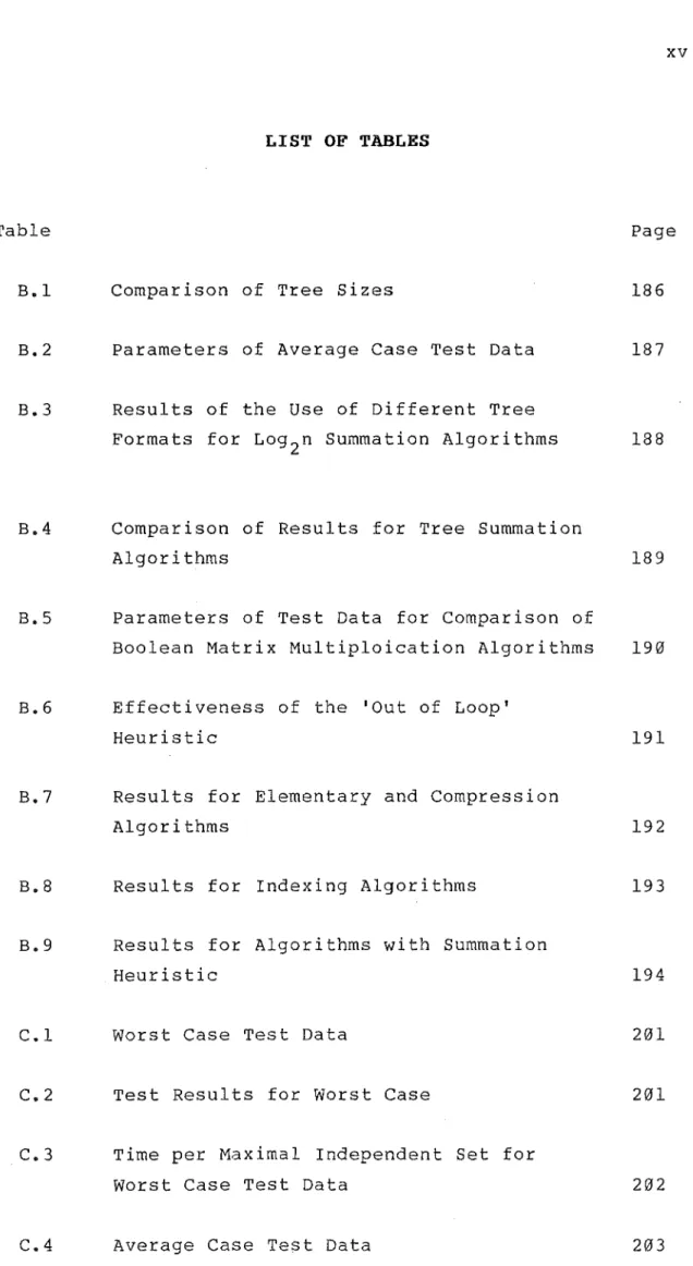
Example 2.4
Figure 2.4 shows the Adjacency List and Edge List for the graph shown in Figure 2.1.
N ( 1)
=
2,10 1: (1,2) 11: (7,10) N ( 2)=
1,7 2: (1,10) 12: ( 7, 9) N (3)=
4,8,9,10 3 : (2,7) 13: ( 3, 8) N ( 4)=
3,8,9,10 4: ( 5, 10) 14: ( 4 1 8)N ( 5)
=
7,10 5: ( 5, 7) 15: (3,4) N ( 6)=
9,10 6 : (4,10) 16: ( 61 9) N ( 7)=
2,5,9,10 7: (8,10) 17: ( 3 1 9)N ( 8)
=
3,4,9,10 8 : ( 3, 10) 18: ( 8, 9)N (9)
=
3,4,6,7,8,10 9: ( 9 1 10) 19: ( 4 1 9)N(l0)
=
1,3,4,5,6,7,8,9 10: (6,10)(a) (b)
(a) ADJACENCY LIST FIG 2.4
(b) EDGE LIST (end of example)
2.4 GRAPHS AND BOOLEAN MATRICES
Definition 2.25
A closed semiring is an algebraic structure (S,+,.,0,1) on a set S which defines two binary operations, denoted by + and
1. a+b is in S and a.b is in S (+ and • are closed)
2. (a+b)+c = a+(b+c) and (a.b) .c = a. (b.c) (+ and • are associative)
3. a+b = b+a (+ is commutative) 4. a+a = a (+ is idempotent)
5. a+0 = 0+a = a for every a in
s
(0 is the + identity)6. a.l = l.a = a for every a in
s
(1 is the.
identity)7. a.0 = 0.a = 0 (0 is an annihilator)
8. a. (b+c) = a .b· + a.c and (a+b) .c = a.c + b.c (. distributes over +)
9. If a
1,a2, •• ,ai, ••• is a countable sequence of elements then a1+a2+ •• +ai+ ••• exists and is unique 10 • • distributes over countably infinite sums as well
as finite sums
A closed semiring of particular importance for this work is the semiring S'=({0,1},+,.,0,1) with addition and multiplication tables as follows:
f:
0 1Let G=(V,E) be a directed graph, where V={v
1,v2, •• ,vn}. For a labelling function L: (VxV)->{0,1} over the elements of S' such that
L (v. , v . )
=
1 J
if (v.,v.)
1 J
otherwise
is in E
the graph G can be represented by the nxn matrix AG whose ijth entry is L(v.,v.). The matrices AG are also defined
1 J
over the semiring S'.
2.5 TREES
Trees have been defined and analysed by Knuth [1973] and their use in many algorithms is described by Aho, Hopcroft and Ullman [1974].
Definition 2.26
A connected acyclic directed graph is a directed tree if 1. There is exactly one node, called the root, which no edges enter.
2. Every node except the root has exactly one entering edge.
3. There is a unique path from the root to each node. A tree with n nodes has exactly n-1 edges.
Definition 2.27
descendents is called a leaf.
Definition 2.28
The depth of a vertex v in a tree is the length of the path from the root to v. The height of a vertex v in a tree is the length of a longest path from v to a leaf. The level of a vertex v in a tree is the length of the path from a leaf to v.
Definition 2.29
An ordered tree is a tree in which the children of each node are ordered. A ordered binary tree is an tree such that:
1. each child of the node is distinguished as either the left child or the right child and
2. no node has more than one left child and one right child.
An ordered log tree is an tree such that no node has more than log
2n children.
When drawing an ordered tree, the children of each vertex are assumed to be ordered from left to right.
Definition 2.30
2.6 PROBABILITY DISTRIBUTION
A probability distribution for random graphs is used in the ·analysis of the average time complexity. Erdos and Renyi
[1959] present two equivalent graphical distributions.
Definition 2 .. 31
G are the graphs of n vertices where each edge is chosen n,p
independently of other edges and is present with probability p.
G are the graphs of n vertices and N edges where n,N
the N eges are distributed at random through n(n-1) possible edges.
The complexity analysis of Chapter 5 will use the first distribution. For an adjacency matrix A of a graph G=(V,E),
the probability that an edge exists is
Probability(a .. = 1) = p
lJ
and the probability that an edge does not exists is given by
Probability(a .. = 0) = 1-p
lJ
Probability(k independent edges exist)
=
pkand the probability of k independent edges not existing is
Probability(k independent edges not existing)
=
(1-p)kFurthermore, the probability of m edges existing from a partition of the graph that has z possible edges is
Probability(m edges in a z partition)
=
(z) m z-m
m
p (1-p)2.7 MAXIMAL INDEPENDENT SETS
Definition 2 .. 32
A set
cs;v
such that for all v,w· Ec
implies (v,w)Jl
E is an independent set. If C is not contained in any other independent set then C is called a maximal independent set. The set C'C V such that for all v,w inC implies (v,w) in E is a complete subgraph. If C' is not contained in any other complete subgraph then C' is a clique.c ( n)
=
n=0 (mod 3) 4*3(n- 4 )/ 3 n=l (mod 3) 2*3(n- 2 )/ 3 n=2 (mod 3)
There exists only one (not including all possible isomorphisms) such graph for each value of n. The minimum possible number of independent sets in a graph is one and the graph has n vertices and 0 edges.
The complements of these graphs will have the same number of maximal independent sets as cliques in the original graphs, and this will also be the maximum possible number. For any value n, the graphs ·contain j_n/3_j disjoint polygons on three vertices and, if n is not a multiple of 3, the remaining vertices are connected but disjoint from the polygons of the graph. These complement graphs will be used to test algorithms for finding all maximal independent sets of a graph and the original graphs will be used to test algorithms for finding all cliques of a graph. The graphs will be collectively called the Moon-Moser graphs.
However, these graphs give no indication of the average number of independent sets in a graph, or of the probability of the graph's occurrance. Matula [1970] and Bollobas and Erdos [1976] have studied complete subgraphs and cliques in random graphs. Bollobas and Erdos use the random graph G on
n
n vertices, where each edge is present with probability p independently of all other edges, where 0
<
p<
1 and p is fixed. If Z =z
(G ) is the number of cliques of order r inr r n
then
=
1d(n)
=
2*logn+
O(logl/plogl/pn) log(l/p)Bollobas and Erdos state
"that cliques of order essentially greater than dn are unlikely to occur • • and that cliques of order roughly less than l/2dn are also unlikely to occur, but every other value is likely to be the order of a clique • • • that the orders of cliques occurring are a1most exactly the numbers between •
• • -l/2d(n) and d(n)".
Since Probability(r given vertices
r n-r (r)
= (
1-p ) p 2form a clique in G )
n
the expected number of cliques of order r in G
n
expectation of Z ) is
r
E(Zr)
(the
Then, the expected total number of cliques in the random graph Gn' will be the sum of the expected number of cliques of each possible size.
d
E(c) =
I:.
E(Zr) r=l/2d=
"""'2log l/pn
+
0 (log l/plog l/pn) ( )LJ
(~)
(
l-p r) n-r p~
Clearly, E (c)
<<
3n/ 3 •Thus, the bound for the expected number of cliques or maximal independent sets in the random graph is polynomial and much less than the exponential bound for the worst case, however the number is still very large for small n.
Example 2.5
The graph shown in Example 2.1 has the following independent sets.
(2,10) (1,5,9) (2,5,9) (1,3,5,6) (1,3,6,7) (1,4,5,6) (1,4,6,7) (1,5,6,8) (1,6,7,8) (2,3,5,6) (2,4,5,6) (2,5,6,8)
(a)
9
(b)
(a) THE 12 MAXIMAL INDEPENDENT SETS OF A
(b) GRAPH ON 10 VERTICES AND 19 EDGES (end of example)
CHAPTER 3
A SURVEY OF GRAPH REPRESENTATION
3.1 INTRODUCTION
All non-topological representations of a graph are based on the implicit assumption that the elements of the graph can be arbitrarily labelled. Usually the vertices of the graph G=(V,E) with n=jVj and m=jEj, are labelled with the natural numbers l •• n and the edges are labelled with the natural numbers l •• m. The traditional graph representations used prior to the application of computing are based on the above assumption and have been successfully transfered to computer algorithms to give the best known representations for some graph problems.
Two closely related methods for solving graph problems, decomposition and shrinking, are related to the algebraic concepts of subalgebra and homomorphism. Both methods are generally termed decompositions. These methods are not restricted to graph problems, as decomposition techniques have been presented for varying combinatorial classes. There are a number of combinatorial optimisation problems which can be solved more efficiently on the composition graph by solving similiar problem instances on the smaller graphs. Decompositions of graphs, based on both decomposition and homomorphisms of graphs, and their application to graph algorithms are surveyed in this chapter.
3.2 REPRESENTATION OF GRAPHS
The graph representations discussed in Chapter 2, using matricies and l i s t s , are conveniently adapted to data structures within conventional programming languages using, in the simplest form, only arrays. Furthermore, in section 2.5 the relationship of adjacency matrices to the closed semiring of boolean algebras was detailed, so the adjacency matrix can be manipulated according to the laws of algebra which are far better established than the laws of graph manipulation.
Matrix or l i s t data structures are efficient and 'natural' representations of some graph problems. Multiplying boolean matrices is equivalent to computing the transitive closure
less laborious methods for computing the closure than computing the successive powers of the adjacency matrix, and many path problems are algebraically equivalent to the determination of one or more elements of the weak or strong closure of an adjacency matrix [Carre, 1979]. The solution methods discussed by Carre range from substitution through Gaussian and Jordan elimination to Dijkstra's algorithm and a l l use matrix or l i s t data structures. The theoretical framework used for the formulation and solution of path problems is a path algebra. Path algebra are defined for accessible sets, shortest paths, critical paths, most reliable paths, paths of greatest capacity and enumeration of paths in a graph. Mahr [1981] surveys shortest path problems and their general solution techniques and the adjacency matrix also dominates these solutions.
A matrix representation does not give the best known solutions for a l l graph problems, for many of which an efficient computer representation requires data structures tailored to the problem area. The history of algorithm design has many milestones marked by the development of new data structures which have led to new and efficient algorithms [Aho, Hopcroft and Ullman, 1974]. The most recent was the development of the Fibonacci-heaps applied to shortest path problems [Fredman and Tarjan, 1984] and since used for efficient algorithms for finding minimum spanning trees, maximum weighted matchings and optimum branchings
Among the earliest data structures to have a fundamental effect on the design of efficient algorithms was the tree. Nievergelt [1979] describes trees as:
"Thus, trees have emerged as THE class of l i s t structures which are most widely used, and are understood best from a theoretical point of view. Knuth collected and c l a s s i f i e d the accumulated knowledge on data structures [1968,1973] • Of all the data structures considered, trees claim the lions share of the space."
The tree data structure is closely linked to an algorithm that has been used extensively to systematically search a graph, the depth first search which derives an underlying tree substructure from the graph. The tree created by depth first search was termed a palm tree with fronds. The fronds are back links in the tree and they determine the connectivity of the original graph. Depth first search has been used to find the biconnected components of an undirected graph in O(m) time [Hopcroft, 1971], the triply connected components in linear time [Hopcroft and Tarjan, 1973], and the strongly connected components of a graph in 0 (max (n,m)) time by adding cross links [Tarjan, 1972]. It has also been used in the path addition algorithm for testing graph planarity in linear time [Hopcroft and Tarjan, 1974], the best known algorithm for finding dominators in graphs [Tarjan, 1974] and a test for flow-graph reducibility in linear time by adding path compression which redefines the root of the tree to achieve a balanced tree structure
In general, problems on trees are simpler to solve than problems on more general graphs. Indeed, some NP-complete problems have polynomial time solutions when restricted to trees.
The identification of particular properties of a class of graphs establishes a restriction on the complexity of the graphs that can be used to develop efficient algorithms for that class of graph. This is apparent in the clique problem. The COVERING BY CLIQUES problem, finding all the cliques in a graph, is NP-complete. The PARTITION INTO CLIQUES problem, is solvable in polynomial time for graphs containing no complete subgraphs 6n 3 vertices, for circle arc graphs, chordal graphs and for comparability graphs, and the CLIQUE subgraph problem is solvable in polynomial time for graphs obeying any fixed degree bound, for planar graphs, edge graphs, chordal graphs, comparability graphs, circle graphs and for circle arc graphs. [Garey and Johnson, 1979].
3.3 GRAPH DECOMPOSITION
efficient solutions. The algorithms of Gabow, Galil and Spencer [1984] discussed in section 3.2, use Fibonacci-heaps to maintain and merge the components of a graph and from this some very fast and efficient contraction algorithms have been developed.
The use of totally ordered label sets implies an ordering relationship within the graph which does not exist. Furthermorei since any labelling is valid, any ordering relationship can be established. This reordering is equivalent to the graph isomorphism problem. The graph structure is lost within these representations as are all graph parameters except the number of nodes and the number of edges and even the latter is lost in an adjacency matrix. Frucht [1970] introduced a notational representation of graphs that is independent of any labelling. The graph is represented by the orbits under the cyclic subgroups of the automorphism groups of the graph. The method is succienct and readily translated to computer storage.
NP-Complete
IU
Isomorphism Complete
n
NPIU
Automorphism Complete
n
NPIU
p
THE COMPLEXITY HIERARCHY FIG 3.1
3.4 GRAPH HOMOMORPHISM
More successful attempts at decomposing a graph have been based on the homeomorphisms and homomorphisms of a graph. If part of a graph is shrunk to a single vertex and a problem is solved on the shrunken graph then the solution on the original graph can be computed from the solution on the smaller graph. The shrinking corresponds to taking a homeomorphic image of the graph. A homomorphism usually can be defined only on the paths of a graph, rather than the edges of a graph.
The usual graph homeomorphism is an adjacency homeomorphism as used in Kuratowski's theorem. Perl [1980] used this to define a reachability homomorphism on directed graphs. However, this definition allows the introduction of new reachablities and Ebert and Perl [1981] point out that this problem has not yet been solved.
Sabuddissi [1961] defined the X-join of a family of graphs. The X-join is a composition operator on graphs that obtains, from the graph X, a composition graph by substituting each vertex of X by the graph Gx in the set. Every graph is isomorphic to an X-join of some family of graphs, but possibly only a trival set. That is, either X is trival or all Gx are. If a graph is isomorphic to an X-join of some family of graphs and both X and some member of the family are non-trival then the graph is decomposable.
James, Stanton and Cowan [1972] reported an algorithm for decomposing graphs with respect to the X-join. The algorithm requires O(n4) time.· Habib and Maurer [1979] presented an O(n3) algorithm for decomposing undirected graphs.
Pfaltz [1972] defined a homomorphism on directed acyclic graphs, and showed how to retain the ability to reconstruct the original graph from the sequence of contracted graphs. The homomorphism developed from the study of an equivalence relation, over nodes of the graph, that is dependent on preserving adjacencies.
operator domain consists of its relations.
A similar approach was used by Cardon and Crochmere [1982]. They further gave an algorithm for finding the graph homomorphism in O(m*log
2n).
Cunningham and Edmonds [1980] generalises these theorems in a unifying decomposition theory. Non-separable graphs are defined and a simple decomposition operator is developed from which a unique minimal decomposition can be defined. Cunningham [1982] presents the composition for digraphs and shows that a general decomposition theory can be applied to the resulting digraph decomposition which is unique as each member of the decomposition is either not decomposable or belongs to a class of special digraphs which are completely characterised. Algorithms for the decompostion requiring O(n4) time and O(m) space are also presented. For special classes of graphs the complexity is reduced to O(n3) time and order O(n+m) space.
3.5 SUMMARY
Many graph representations translated easily to computational structures for the solution of graph problems and data structures such as trees which are extensively used in other areas of computing have been used to develop the best known solutions for many graph problems.
The search for specifically designed g~aph structures, and the theoretical development of graph decompositions which has been the subject of much research, have not, in general, led to applications in graph algorithms. In practice, decompositions have·generally been restricted to certain classes of graphs, while graph representations based on the automorphism or clique structure of a graph are also restricted to the graphs which do not require exponential time to find the graph structure.
CHAPTER 4
A DECOMPOSITION ALGORITHM FOR
SHORTEST PATHS ON NETWORKS
4.1 INTRODUCTION
Many specialised problems within the general framework of path problems have been studied. Christofides [1975] ~nd Carre [1979] give comprehensive studies of the shortest path problem and algebraic path problems respectively. The most common forms of shortest path problems are the 'all pairs' and 'single source' problems. The problem studied in this chapter is a variation of these shortest path problems to find the shortest paths for a selected set of vertices in the network.
paticular flow may exist, and to change between these may also incur extra costs. In many applications within transportation studies only a subset of the distance matrix which is output by an all pairs shortest path algorithm is required. Typically, transportation networks contain many hundreds of vertices and only a representative sample of some 5 to 10 percent of these vertices will be required in a --shortest paths matrix. Clearly, generating the all pairs solution or a multiple single source solution and extracting a submatrix will involve calculations on many otherwise unused vertices in the network.
Cunningham [1982] states that:
"There are a number of combinatorial optimisation problems which can be solved (more efficiently) on the composition graph by solving similar problem instances on the smaller graphs."
the all pairs shortest path matrix of the compressed network can then be combined in the third stage. An algorithm is presented that generates a single pair shortest path on the composition network in linear time, so for any selected set S of vertices of ~ize s=ISI, the shortest path matrix for the set can be generated in O(s2) time.
This chapter also presents the application of the decomposition to transportation networks. The decomposition presented in this chapter is valid for both directed and undirected graphs.
4.2 DECOMPOSITION OF A NETWORK
In this section a decomposition is defined on networks. The decomposition is similar to the homeomorphism used by
Definition 4 .. 1
Let G=(V,E) be a network. Divide the vertices of G into two classes:
(1) the simple vertices are adjacent to exactly two other vertices and either r+(v)(~r-(v)
=
1 or+
)
-r ( v ) { =/ r ( v )
=
2 •(2) the link vertices are the remaining vertices in the network.
The set of all link vertices of G is denoted by L.
Definition 4.2
The edges of the network are partitioned into simple paths between a link vert~x x and a link vertex y in G and all vertices in the path other than x and y are simple vertices and for every pair of simple vertices v. and v. in the same
1 J ')
simple path partition, r+(v.)
=
r+(v.) and r-(v.)=
r-(v.).1 J 1 J ')
The edges and vertices in each partition are called the branches of G. Divide the branches of G into three classes:
(1) the simple paths of length 1 are the trivial branches of G.
(2) the simple paths of length greater then 1 which are polygons, that is link vertex x
=
link vertex y, so the edges form a cycle from a link vertex x L back tox.
Each branch of a network starts at a link vertex. If it is a trivial branch then there will be exactly two vertices (both link vertices) and either one or two edges in the branch. If the branch is a connecting branch or a polygon it will have an edge to an adjacent simple vertex and the branch will include the simple path from the starting link vertex through simple vertices until any other link vertex is reached. If there is an edge from the simple vertex to the starting link vertex then all simple vertices in the branch will include edges incident to both adjacent vertices.
Example 4.1
Figure 4.1 shows a p·ortion of a transportation network that includes 5 link vertices and 9 branches, 1 of which is a polygon and 8 connecting branches. The bidirectional edges of the network are shown as undirected edges in Figure 4.1.
The link vertices of Figure 4.1 are {9054,9055,9056,9057,9058,9059}
The branches of a network include vertices and edges. Two branches of the network portion of Figure 4.1 are shown in Figure 4.2. These are the branches whose vertices are:
1'0 0 i:tl ~ 1-1 0
z
0 i':j>
~~
z
1:/l 1'0 0 ~ ~>
~ 1-1 0z
z i::j ~ ~ 0 ~ ~ i':j 1-1 G'l ~•
1-'80~
/-...*--807/~
~*~
809/
~·---
773~
__/
.
~
*-....____ .;--
:>
8 0 2810f*
~
("I
801*
8/
81
fs:_
7~=---;·
794/0~
- - - 775/*
~·
/776* - - * - d 796
- - - 5 • 793
79 2 *
---~* -~-*
\,779
*
791 875~
779* ---- * -
0\9
0 5 7 9 0 5 6 ' \ 7 8 0798 788
·~
_;. 781787
·~.
~·782
~
---*
7837 8 6
*
'--....*---* 7 8 4 818 817*
*
( 819
\
\~21
*
822\
825 824
*~
23[*-~~
9059826 827 785
*'"'
The vertices of the remaining branches which are shown completely in Figure 4.1 are:
{9054,775,776,777,778,9055} {9055,875,790,791,9056} {9056,792,9057}
{9056,793,794,795,796,9058} {9057,799,798,797,9058}
{9054,800,801,802,803,773,804,805,806,807,808,809,810, 811,813,814,9058}
{9058,815,816,817,818,819,821,822,823,9059}
9057 9055
0 0
788
!"-...
\
77 9 ""' ""' 7 8 0 825 824'k+-'k• " " '
78 7
*
*""-~
*--*
781786
*,
*--*~
782'*--0 9059
*-*--/
826 827 785 784
TWO BRANCHES IN THE NETWORK FIG 4.2
(end of example)
Definition 4 .. 3
The decomposition can now be defined on the vertices and edges of the network.
Definition 4.4
A decomposition D of a network G=(V,E) divides the vertices and edges of G into the branches of G. The components of the decomposition are each of the branches of G.
Each distinct branch of the decomposition is itself a network. Several theorems on the nodes and branches of a graph were proved by Tutte and these extend naturally to the link vertices and branches defined on a network.
Theorem 4.1
Let X be any branch of a graph G. Then
I
V(X)n
LI
<=
2. If X is incident with two distinct (nodes) link vertices x and y of L, then X is a simple path with ends x and y. In the remaining case X is a polygon.Proof. Due to Tutte. (end of proof)
By theorem 4.1 the number of link vertices of G incident with a given branch X is either 2, 1 or 0. In the first case the branch is a simple path joining two link vertices. In the second case the branch is a polygon and there is only one link vertex in the branch. The third case cannot occur
Theorem 4.2
Let G be a graph without divalent edges. The graph H whose vertices are the (nodes) link vertices of G and whose edges are the branches of G is a true graph and there exists an isomorphism f of G onto H. The graph H is the branch-graph of G.
Proof. Due to Tutte. (end of proof)
From theorem 4.2 i t is possible to show that the decomposition of definition 4.3 is sufficiently general to apply to all networks~
Theorem 4.3
For all networks G=(V,E) there exists a decomposition D of G onto the branches of G.
Proof.
Each vertex of a network is either a simple vertex or a link vertex by definition 4.1. Every edge in a network either connects two link vertices in which case i t is a trivial branch, or i t connects a simple vertex with another simple vertex or a link vertex, in which case i t is on a simple path that is either a polygon or connecting branch of G. Every vertex and edge of any network exists on a branch of the network and the branches of G form a decomposition of G.
Tutte defines a homeomorphism f of a graph G onto a graph H as a pair {g,h}, where g is a 1-1 mapping of the (nodes) link vertices L(G) onto L(H) and h is a 1-1 mapping of B(G) onto B(H), such that a (node) link vertex x is incident with a branch X in G if and only if gx is incident with hX in H. The relationship between a graph G and its branch graph is a homeomorphism and so is valid for all graphs, although in the trivial case L=V and the edges of the branch graph are simply the edges of the original graph. Tutte defines the properties of the homeomorphism. These include the existence of an identity homeomorphism and an inverse homeomorphism. The extension to a network retains the homeomorphic relationship between a network G and its branch graph and t h i s graph is unique. So, the components of the decomposition are unique and irreducible.
Theorem 4 .. 4
Every network has a unique decomposition D consisting of the branches of G and every branch br in B is irreducible.
Proof.
A branch of a network G is a simple path from a link vertex x to a link vertex y. If x and y are distinct then the branch must have at least one edge. If x=y then the branch is a polygon of length
>
1, so must have at least one edge. The branches of G partition the edges of G, so no edge can occur in more than one branch. So, each branch of G is uniquely defined by the edges i t contains and the decomposition D is unique.of br, namely V(b ) - (V(b ) n.L), are simple vertices. As
r r
every branch of a network must contain at least one edge and be a simple path between link vertices, there is no other branch in b so b is irreducible.
r r
(end of proof)
The final theorem that must be proved on the decomposition is that the original network can be reconstructed from the components of the decomposition, so a composition on the branches of G must be defined.
Definition 4.5
Let b
1 and b2 be networks having vertex sets V(b1) and V(b2) and edge sets E(b
1) and E(b2) respectively. A composition of b
1 and b2 is the composed network
N
=
bl o b2=
(V (bl) U V (b2) , E (bl) U E (b2)) • IfI
V (b1) n V (b2) 1
>=
1 then N is a connected network.Theorem 4.5
The original network G can be reconstructed from the components of the decomposition B.
Proof.
Each branch of G is a network and so the composition of definition 4.4 may be applied to two branches of G to form a composed network. Since the branches form a partition on the edges of G, no edge will occur more than once in a composed network. If the branches contain a common vertex, i t will only occur once in the union V(b
of G will combine all the edges of G that have been partitioned by the branches. Since the network is connected every vertex will be the end-point of some edge, and so all vertices will be included in the composition of all the branches of G.
(end of proof)
4.3 A COMPRESSED NETWORK
For the solution of shortest path problems that will be presented in this chapter, the branch graph of Tutte although i t extends to a network, will be altered to give a more efficient compressed network. The compressed network of definition 4.7 differs from the homeomorphism of Tutte by the removal of the polygons from the branch graph of G.
Definition 4.6
For each path in a connecting branch b c of a network G, from a link node X to a link node y, define a directed link edge PC
=
(X' y) from X to y. The cost of the new edge c(p ) is the sum of the costs of the edges of path in thec
branch be. For the set B of branches of G, the set of edges pc is denoted by P. If there is more than one link edge
=
(X 'y) then the cost of the edge (X 'y) isDefinition 4.7
A network formed on the link vertices of the network G=(V,E) is the compressed network Gc=(L, E(L) U P). The vertices are the link vertices L and the edges are the edges of the subgraph formed on L (equivalently the trivial branches of G) plus a directed link edge pc replacing every path in the connecting branches of G. The costs of the edges of G are:
c
(1) if e=(x,y) for x,yE L and e
E
E and e = ( x, y) for cx,yEL and ecEE(L) then c(ec)=c(e). ( 2 ) if p EP then c(p )=
c c
L
c (e) for all e in the simple path b •c
Example 4.2
9058
L
<
1 9 0 5 5 _ /~. ~---90-5-7°----9~-56---Q
0
9059
A PORTION OF THE COMPRESSED NETWORK FIG 4.,3
The compressed network of the network portion shown in Figure 4.1 is shown in Figure 4.3. The vertices of the compressed network are the link vertices of the original network, namely {9054,9055,9056,905,9058,9059}. Note the
the compressed network. (end of example)
The size of the compressed network is determined by the original network and the number of link vertices i t contains.
Theorem 4.6
Let
G=(V,E)
be a network with n=
lVI
the number of verticesand m
=
lEI
the number of edges in G. If the number of link vertices in G is t , then the number of vertices in the compressed network is t and the number of edges u ism-2*(n-t+l)
<=
u<=
m-(n-t)Proof.
The vertices of the compressed network are the link vertices of G, so there will be t vertices in the compressed network. If a branch of G is a trivial branch then for each edge in the branch (forward and/or backward) there will be exactly one edge in the compressed network. If a branch of G is a polygon containing p simple vertices and 1 link vertex then either p+l or 2*(p+l) edges of the original network will not occur in the compressed network. A connecting branch of G containing p simple vertices and 2 link vertices with p+l edges will be replaced by 1 edge and if the branch contains 2*(p+l) it will be replaced by 2 edges. A compressed network with t link vertices has n-t simple vertices deleted so at least n-t edges are deleted and at most 2*(n-t+l) edges are deleted.
The decomposition that has. been defined provides for two essential requirements; namely, that the components of the decomposition are unique and irreducible and that the original network can be reconstructed from the components of the decomposition. The algorithm to generate the compressed network that has been defined on the components of the decomposition will also calculate the costs of the shortest paths on the components of the decomposition and is given in Algorithm 4.1.
A planar network is sparse and so will be presented most efficiently as an adjacency l i s t . The costs of the input network G may either be presented as a matrix or attached to the adjacency l i s t . Every simple vertex occurs in only one branch of the network and on at most two simple paths, one forward and one backward. Every edge will be traversed exactly once forward and once backward by the algorithm, so O(m) time will be required.
Algorithm 4.1
Generating the Compressed Network and the Shortest Paths of the Components of the Decomposition.
Input: A network G and the costs c associated with each edge in the network.
Method:
Find the link vertices of G: for every vertex v. in G
1
if not ( (r- (vi)
=
r+ (vi)=
1) or (r- (vi)=
r+
(v.)=
2)) 1then v. is a link vertex
1
Find the costs for the link edges and the components: for every link vertex vi do
for every v., in r+(v.) do begin
1 1
follow a simple path
calculating the cost of the shortest path from vi to every simple vertex in the path
(and ultimately the cost of the link edge) until another link vertex vi" is reached
if the path is not a polygon then
store the total cost of the path as the cost of the link edge (v.,v.1 1 11 ) in the compressed network
trace backward through the simple path from v. 11 to v.
1 1
end
calculating the cost of the shortest path from every simple vertex in the path to until link vertex v.
1 is reached
(end of method)
v. " 1
vertex with the cost of the shortest path from the simple vertex to the end link vertex will completely define the path direction.
Two distinct branches b
1 and b2 may occur with the same link vertices; that is jV(b1 )
n
V(b2 ) 1
=
2. For all simple vertices in both b1 and b2 the start link and end link of the vertex will be the same although they do not occur in the same branch. During the decomposition process each branch of simple vertices is traced, so if two vertices are in the same branch they may be labelled with the same path identification. Thi~ will distinguish between two vertices with the same link vertices, but on different branches of the decomposition.
Example 4.3
Figure 4. 4 (a) shows the simple vertices on a forward and backward path between two link vertices 9055 and 9057. The shortest paths from each link vertex to the simple vertex 785 are shown in Figure 4.4 (b) as the 'cost_to_vertex', and the shortest paths from the simple vertex to the link vertices are shown as the 'cost from vertex'.
()~
...
----...---."-·~-~:--;