Lies, damn lies and differential equations

University of Warwick institutional repository: http://go.warwick.ac.uk/wrap This paper is made available online in accordance with

publisher policies. Please scroll down to view the document itself. Please refer to the repository record for this item and our policy information available from the repository home page for further information.

To see the final version of this paper please visit the publisher’s website. Access to the published version may require a subscription.

Author(s): David Tall

Article Title: Lies, Damn Lies ... and Differential Equations Year of publication: 1986

Lies, Damn Lies ... and Differential Equations

David Tall

Mathematics Education Research Centre University of Warwick

COVENTRY CV4 7AL

The title of this article is a misquotation of Disraeli's comment on statistics, but there is every reason to apply it to the way we currently teach differential equations at A-level. The problem is that we try to make the theory ‘easier’ for the students by concentrating on simple special cases, not delving too deeply into the technicalities. This tactic has two fundamental flaws. First, the oversimplification of the theory can lead to misrepresentation and falsification of the mathematical facts. Second, the presentation of the theory as a number of special cases may lead to the mistaken belief that differential equations are solved by a number of isolated techniques (separation of variables, exact solutions, integrating factors, and so on), without any perceivable overall rationale binding the theory together.

The arrival of the computer gives us the opportunity for a fresh look at the theory to give a clearer insight into the fundamental ideas. Using simple numerical methods it is possible to sketch the solutions of differential equations, showing visually how the theory works and under what circumstances there are likely to be difficulties.

A terminological inexactitude

The simplest kind of differential equation is of the form:

dy/dx=f(x)

and a solution is a function I(x) such that I'(x)=f(x). The function I(x) is often called the "improper integral" of f(x) or, more appropriately, the "antiderivative", found by reversing the process of differentiation.

For example, if

then one solution is I(x)=x2 _{and a more general solution is x}2_{+c for some constant c.}

It is common practice in A-level texts to move quickly on to the more general function f(x)=xn_{, to announce that the general solution of}

dy/dx=xn ₍₁₎

is (for n≠–1)

y=xn+1_/(n+1)+c.

Regrettably, there is a logical flaw in the argument, and a serious one at that. Suppose that I(x) is one solution of a differential equation (1).

Let P be the statement ‘J(x)=I(x)+c’ and Q be ‘J(x) is a solution of (1)’ then P implies Q (by differentiation), but it does not follow that Q implies P. The converse fails when n is a negative integer, as can be seen by considering n=–2.

The solution of the equation

dy/dx=1/x2 ₍₂₎

is a function y=I(x), whose graph has gradient I'(x)=1/x2 _{everywhere. This may be}

represented in a picture by drawing short lines through a selection of points (x,y), such that the gradient of each short segment is 1/x2 _{(taking the value of x at the midpoint). The}

resulting picture is shown in figure 1.

A solution of the differential equation (2) is found by tracing a curve y=I(x) in such a way that the curve always has gradient 1/x2_{. A sketch of the solution curve may be built up}

numerically by starting at any point (x,y), moving a short distance in the direction with gradient 1/x2_{, then recalculating the gradient at the point reached and repeating the process.}

(An even more accurate method is to calculate the gradient at A=(x0,y0), taking a temporary

step a short distance in this direction to B=(x1,y1). Instead of moving to this point,

recalculate the gradient here, then move back to A, and take a step in the direction found by averaging the two calculations. It is this improved version of the calculation that is used in

Graphic Calculus II5 _{to give a more accurate picture.)}

A typical solution is traced in figure 2. In following the directions of the short line segments, the solution curve does not cross over the y-axis.

Figure 3 : A solution of the differential equation

We need to be a little more careful about what we mean by a solution of a differential equation. One possiblity is what I shall term a connected solution, in which the differential equation is considered to describe the continuous motion of a point (x,y). Such a solution curve is in one piece and will not cross the y-axis. If it is to the left, it will be in the form

I(x)=–1/x+c for x<0.

The second possibility is to allow the solution to be a more general function. In this case it is permissible to move over to the other side and independently draw another part of the solution curve to give the more general form

where the constants c and k may be different.

The necessity of spelling out the difference between these two cases may seem a small matter. Perhaps it is. But in mathematics, that most logical of sciences, from such small deficiencies may grow fundamental weaknesses in the theory. When I was writing my first mathematical textbook, my friend and mentor, Walter Ledermann, told me that in teaching you need not tell the whole truth, but you should never lie...

When the ‘arbitrary constant’ is used in more general differential equations, the problem is compounded.

Blind manipulation of formulae

A recent A-level question asked candidates to:

obtain the general solution of

ydy_{dx sec2x = 1–y}2_{. (3)}

A typical solution might involve separating the variables in the form

y

(1-y2₎ dy = cos2x dx

and integrating to obtain the ‘general solution’:

–ln|1–y2_{| = sin2x+c. (4)}

But what does this solution mean? Is this truly the ‘general solution’ in the sense that every solution of the differential equation (2) is found by giving c an appropriate value in (4)? In truth it is not, for in dividing by 1-y2 _{one has lost the two functions y=1 and y=–1 which}

are clearly solutions. Formal manipulations performed without care may lead to inaccuracies.

A geometric picture of solutions

Writing the equation in the form

dy/dx = cos2x(1-y2_{)/y (5)}

and drawing short line segments of gradient

cos2x(1-y2_)/y,

gives figure 3. Superimposed on it are a few curves obtained by following the gradient directions using numerical calculations. The curves at the top and bottom give oscillating graphs with y expressible as a function of x but others nearer the x-axis seem to be closed loops. Some of the solutions are explicit functions and others may be implicit...

Figure 3 : Numerical solutions of a differential equation

Vertical tangents

A technical difficulty of some importance occurs with the apparent solutions in the form of closed loops. Wherever y=0 the gradient dy/dx is not defined in (3). For this reason some mathematicians do not allow such loops to be solutions. (See, for example, Neill and Shuard 2 page 146.)

However, if one regards the tangent as a vector (dx,dy), as in an earlier article in this series 3 then the equation, in the form

(1-y2_{)cos2x dx = y dy, (5)}

may be considered as an equation for the direction of the tangent vector. When y=0, this reduces to

cos2x dx = 0

and (for cos2x≠0) this implies dx=0 and gives a vertical tangent direction (dx,dy)=(0,dy). With this interpretation it is possible to consider a point moving right round one of the closed loops.

I acknowledge freely that equations (3) and (6) are not truly equivalent. (For example, one may take cos2x=0 in (6), but not in (3).) But in interpreting differential equations, one should attempt to get the most natural form of the equation. The difficulty clearly arises from the way in which equation (3) is written using the expression sec2x.

Following one’s nose

The idea behind the solution of a first order differential equation

dy/dx=f(x,y)

now becomes plain to see. It is simply a matter of drawing a curve which everywhere has gradient f(x,y).

The slightly more general equation

follows in the same way when f(x,y)/g(x,y) is well-defined and the case g(x,y)=0, f(x,y)≠0 may be conveniently considered as having a vertical tangent.

For example

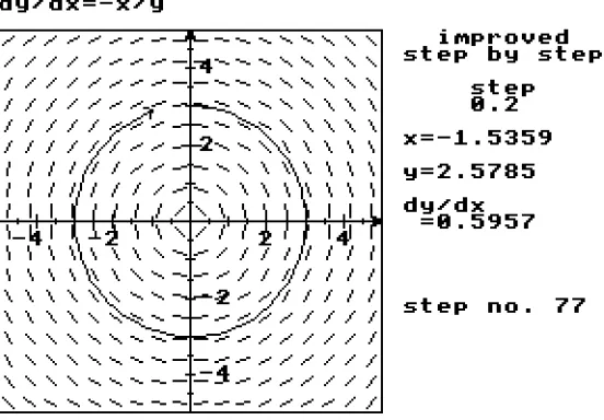
ydy_{dx = -x} (8)

is the differential equation such that the tangent (dx,dy) is in the direction of the vector (y,-x), which is always at right angles to the vector (x,y). The solution curves are therefore circles (figure 4). (Here it is a matter of taste, or convention, whether one is willing to regard equation (8) as being essentially the same as dy/dx=-x/y...)

Figure 4 : A solution of dy/dx=–x/y

The only time when it is not possible to trace a solution of equation (6) is at points where the equation does not define the direction (dx,dy). For example, in equation (1) where y=0 and cos2x=0, or in equation (7) at the origin. Such points are called singularities.

This gives the central idea for solving a first order differential equation:

where the direction (dx,dy) is defined, follow it. The only places where a solution is not possible are where the differential equation has a singularity.

A text-book I favour for its direct and clear approach is Bostock & Chandler1_{. However, I}

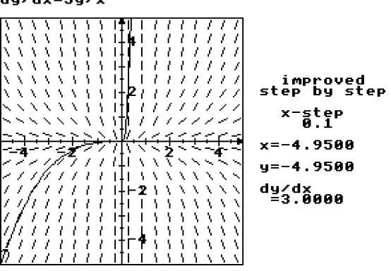
did have problems with my computer program when I tried it out on one of the very first problems on differential equations in the book (page 328):

‘A curve is such that at any point the gradient multiplied by the x-coordinate is equal to three times the y-x-coordinate at that point. If the curve passes through (1,4), find its equation.’

The given condition is written as

x dy_{dx = 3y,} (9)

the variables are separated to give

dy

y = 3

dx

x

and the equation integrated to give

ln|y| = 3 ln|x| + A,

for an arbitrary constant A. Further simplification gives

y=kx3

where k is a constant, and the solution through x=1, y=4 has k=4.

Imagine my surprise when I typed the formula into my differential equations program and attempted to draw a solution (figure 5). The direction diagram clearly shows line segments that follow the shape of cubics in the form y=kx3 _{for k positive, negative, or zero. Yet}

FIgure 5 : A peculiar solution

I was, at first, convinced that there was a bug in the program and spent some time trying to find it. Then I realized that the bug was not in the computing, it was in the analytic solution

as given in the book. Considering the original equation (9) as specifying the tangent

direction of the curve in the form

x dy = 3y dx,

describes the direction everywhere, except at the origin where it becomes

0.dy = 0.dx.

This gives no information about the tangent direction whatsoever. Thus, if one is viewing the solution, in the most general sense, as being any curve whose direction is specified by the differential equation, at the origin there are no restrictions in the words of Cole Porter

-anything goes! A more general solution of the equation is

y= _ kx

3 _{(x< 0 )}

cx3 _(x≥_{0 )}

where the constants k and c may be different.

Simultaneous Differential Equations

Although simultaneous first order differential equations are certainly not part of the A-level syllabus, it is important to look briefly at them numerically to see how they are simple generalizations of the case we have just considered.

Consider the example of a point (x,y) moving according to the two equations:

dx/dt = y

dy/dt = –x

where t is time. Imagine the point (t,x,y) in three dimensions moving along a curve which has tangent direction (dt,dx,dy) determined by the equations:

dx = y dt, dy =–x dt. (10)

The tangent vector is

(dt,dx,dy) = (dt, y dt, –x dt)

which is in the direction (1,y,–x).

Figure 6 : A numerical solution of simultaneous differential equations

has direction (1,y,–x) in (t,x,y)-space. The projection of the second and third coordinates onto the x-y plane gives the circular solution seen earlier. Dividing the equations in (10) one obtains the equation dy/dx = –x/y.

Similar interesting phenomena occur when differential equations for dy/dx are given in terms of dy/dt and dx/dt. For example, the equations:

dx/dt=y, dy/dt = (1–y2_)cos2x

may be seen to reduce to equation (3) by dividing the second by the first. But in this explicit form, they give information as to the speed of the point (x(t),y(t)) moving round solution curves. Figure 7 shows three numerical solutions starting at t=0, x=0 with y successively -1.5, 0, 1.5. The outer ones give part of the original oscillating solutions (and negative t would give the other part), but the inner solution travels round in a loop...

1

2 3

3

2

1

1

2 3

Figure 7 : Three solutions of dx/dt=y, dy/dt=(1–y2_)cos2x

Higher order differential equations

A typical higher order differential equation met at A-level is the second order differential equation

Unlike a first order differential equation, this does not seem to have a direction for each point (t,x). Figure 8 shows a number of distinct solutions drawn (numerically) starting from the origin in different directions. There is no simple direction field with a single direction to follow at each point and the simple idea of ‘following one's nose’ now seems inappropriate.

FIgure 8 : Many solutions of a second order differential equation through one point (in this case the origin)

But this is not so. By introducing another variable for the first derivative,

v=dx/dt,

the original equation may be written as two simultaneous equations:

dx/dt=v

dv/dy=-x.

These are precisely the equations studied in the previous section, with v in place of y. A solution follows the tangential direction (dt,dx,dv) in three-space given by

(dt,dx,dv)=(dt,vdx,-xdv).

Figure 9 : A solution to d2_x/dt2_{=–x using the substitution v=dx/dt in (t,x,v) space}

The general idea of a solution

The process given in the previous section can be applied to many higher degree ordinary differential equations. For instance, given

d3_x

dt3 = sinx

d2_x

dt2 –

dx

dt + cost

the substitutions

v=dx/dt

v=d2_x/dt2

can be employed to transform the equation into the equivalent system

du/dt=usinx–v+cost

dv/dt=u

du/dt=v.

simultaneous projections in (t,x), (t,u), (t,v) planes, giving a geometrical flavour once more.

Theoretically one may cope in the same way with ordinary differential equations of higher order, or with a number of simultaneous differential equations of various orders. This means that the simple first-order case is truly representative of what happens in the more general situation and is therefore worthy of extended study in the early stages.

What to do in future

How will this change what we do in school? It will first make us realize that the formal techniques of solving differential equations taught in A-level are flawed. The new technology for drawing numerical solutions provides the opportunity now to allow students to explore the behaviour of solutions geometrically to gain greater insight into the ideas. In this way we may begin to see how the power of numerical and graphical methods complement those of formal manipulation. In the words of Neill and Shuard (page 147):

The three methods of studying a first order differential equation, the sketching of solution curves, their numerical evaluation, and obtaining explicit formulae for them by integration, all contribute to an understanding of the solution.

References

1. Bostock & Chandler 1979: Pure Mathematics I, Stanley Thorne

2. Neill and Shuard 1982, Teaching Calculus, Blackie.

3. D O Tall 1985: "Tangents and the Leibniz Notation", Mathematics Teaching.

4. D O Tall 1986a: Graphic Calculus II: Integration, Glentop Publishers.